The data we use consists of 10 different stocks from the Dow Jones Industrial Average index (see the next table for an overview). We use the 21 trading days between 06/01/2011 and 06/29/2011. Trading on NYSE and NASDAQ is continuous between 09:30 and 16:00. After aggregating the data into 15-minute time slots, we receive 26 observations every day, and a total of 26 * 21 = 546 observations overall.

All the used stocks are liquid enough to have positive turnover in each time slot throughout the observed period. However, it should be noted that since the model has an additive structure, zero turnover in some of the slots would not cause any difficulties.

The following table is taken from the source http://kibot.com/:

Stocks included in the data set

Out of the 546 observations, we will use the first 520 (20 days) as the estimation period, and the last 26 (one day) as the forecast period. It is important to keep the actual data for the forecast period so that we can assess the precision of our forecast and compare it to the actual realizations.

As an illustration of the data, see Figure 3.1 that depicts the first five days (130 observations) of Alcoa.

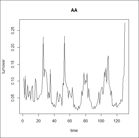
Figure 3.1: First five days of Alcoa turnover

Although every day is a little different, we can clearly see the five separate days indicated by the five U shapes in the turnover graph.

We organized the data in a .csv file with the tickers in the header field. The dimension of the data matrix is 546 x 10. The following code loads the data and prints the first five rows and six columns:

turnover_data <- read.table("turnover_data.csv", header = T, sep = ";") 
format(turnover_data[1:5, 1:6],digits = 3)

The output for the top-left segment of the data matrix is shown below. Given that our data shows turnover values (in a percentage form), and not volume, each value is below unity. We can see, for example, that within the first 15 minutes of the sample, 0.11 percent of the total shares outstanding of Alcoa were traded (see Equation (1)).

     AA    AIG    AXP     BA    BAC      C
1 0.1101 0.0328 0.0340 0.0310 0.0984 0.0826
2 0.0502 0.0289 0.0205 0.0157 0.0635 0.0493
3 0.1157 0.0715 0.0461 0.0344 0.1027 0.1095
4 0.0440 0.1116 0.0229 0.0228 0.0613 0.0530
5 0.0514 0.0511 0.0202 0.0263 0.0720 0.0836

The following code plots the first day of Alcoa turnover. The graph is shown in Figure 3.2.

plot(turnover_data$AA[1:26], type = "l", main = "AA", xlab = "time", ylab="turnover")

We can recognize the U shape of the first day, but we need to rely a little on our imagination at this point. This is because the U shape is a stylized fact that is only observed on a statistical basis.

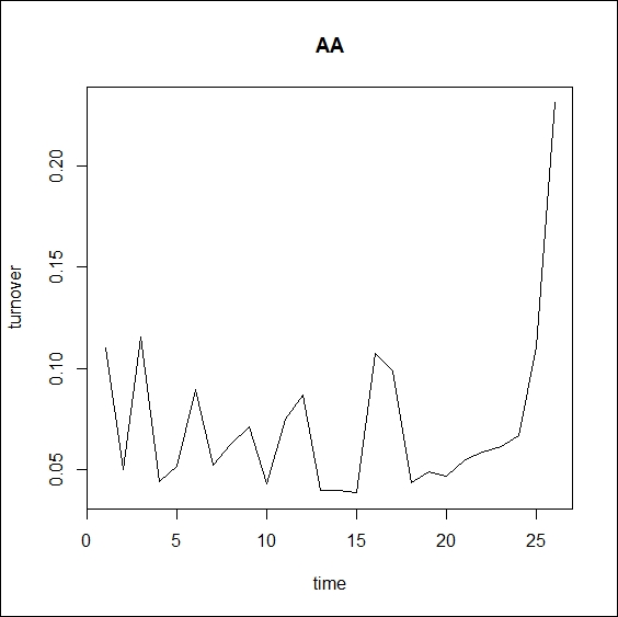
Figure 3.2: First day of Alcoa turnover

We therefore expect the U shape to be more definite on average. The following code plots the average Alcoa turnover throughout the 21 days of the sample. To this end, we transform the first column of the data matrix into a 26*21 matrix, and plot the row averages.

AA_average <- matrix(turnover_data$AA, 26, 546/26)

plot(rowMeans(AA_average), type = "l", main = "AA" , xlab = "time", ylab = "turnover")

The result is shown in Figure 3.3, where the U shape is very clearly drawn.

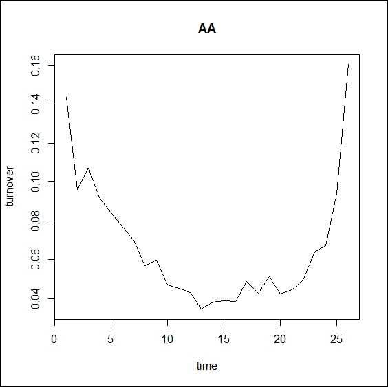
Figure 3.3: 21-day average of Alcoa turnover

Now that the data is loaded, we are ready to implement the model.

The first step is to determine the seasonal component. As mentioned earlier, we will use the first 520 observations for estimation. The following code creates the appropriate sample matrix from the data frame:

n <- 520
m <- ncol(turnover_data)
sample <- as.matrix(turnover_data[1:n, ])

Now, we can start the factor decomposition (see Equations (2) to (6)) of Bai, J. (2003). After creating the matrix (of dimension 520 x 520), we find its eigenvalues and eigenvectors.

S <- sample %*% t(sample)
D <- eigen(S)$values
V <- eigen(S)$vectors

Next, we have to determine the number of factors to use (r). The following code plots the eigenvalues in diminishing order:

plot(D, main = "Eigenvalues", xlab = "", ylab = "")

The result is shown in Figure 3.4, where the first eigenvalue clearly dominates all the others. This means that the variance explained by the first eigenvector explains the majority of the variance, so we choose to use a single factor in our model (). As a rule of thumb, we can use as many factors as the number of eigenvalues that are greater than one, but it always remains a subjective decision.

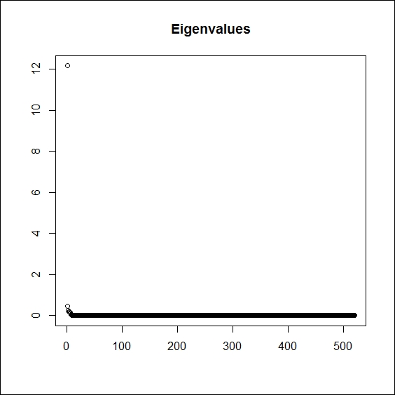
Figure 3.4: Eigenvalues of XX'

Using the eigenvector that corresponds to this largest eigenvalue, we can now compute the estimated factor matrix (see Equation (3)).

Eig <- V[, 1]
F <- sqrt(n) * Eig

Then, we calculate the transpose of the estimated loadings matrix according to Equation (4), and the estimated common (seasonal) component according to Equation (5). Finally, the dynamic (idiosyncratic) component is also calculated (see Equation (6)).

Lambda <- F %*% sample / n
K <- F %*% Lambda
IC <- sample - K

The dynamic component will be forecasted in the following two subsections, but we still need to forecast the seasonal component here. This will be done according to Equation (7).

K26 <- matrix(0, 26, m)

for (i in 1:m) {
    tmp <- matrix(K[,i], 26, n/26)
    K26[,i] <- rowMeans(tmp)
}

The previous code calculates 20-day averages for all 26 slots, dealing with one stock at a time, resulting in a 26 x 10 matrix, including one-day seasonal component forecasts for all 10 stocks.

Now, we have the forecasts of the dynamic component left, which will be done in two different ways: by fitting an AR(1) and a SETAR model.

In this subsection, we fit AR(1) models to the dynamic component. We will need to specify 10 models, one for each stock. The following code performs the parameter estimations:

library(forecast)

models <- lapply(1:m, function(i)
    Arima(IC[, i], order = c(1, 0, 0), method = "CSS"))
coefs <- sapply(models, function(x) x$coef)
round(coefs, 4)

Coefficients are collected in the coefs variable and printed in the following output, rounded to 4 digits. Coefficients need not necessarily be saved (saving the model would be sufficient) because the forecast package has a built-in forecast function, and we will make use of this in the following example:

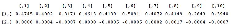
AR coefficients for each stock

library("tseries")arma_mod <- arma(IC[, 1], order = c(1, 0))

So the next step is to produce the forecasts for the next day, that is, for the next 26 time slots using the AR(1) models estimated previously. The following code performs this for us:

ARf <- sapply(1:m, function(i) forecast(models[[i]], h = 26)$mean)

In order to receive the complete forecasts (including both the seasonal and the dynamic components), we simply refer to Equation (11).

AR_result <- K26+ARf

The full forecasts are now stored in the AR_result variable.

The second method for obtaining forecasts of the dynamic component is through a SETAR model. Again, we need 10 different models for each stock. There is also a package in R for SETAR estimation, so the code becomes as simple as this:

library(tsDyn)
setar_mod <- apply(IC,2,setar, 1);
setar_coefs <-  sapply(setar_mod, FUN = coefficients)
round(setar_coefs, 4)

Unlike the AR model, we do have to save the coefficients explicitly for the forecast, which is also done by the previous code. The 4-digit rounded values are printed in the following output:

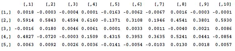
SETAR coefficients for each stock

The five parameters from top to bottom are the following (see Equation (9) for details):

Now, all we have left to do is to forecast the dynamic component for the next 26 time slots using the SETAR model we just described. This is done using the following code:

SETARf <- matrix(0, 27, m)
SETARf[1,] <- sample[520,]

for (i in 2:27){
SETARf[i,] <- 
(setar_coefs[1,]+SETARf[i-1,]*setar_coefs[2,])*
(SETARf[i-1,] <= setar_coefs[5,]) + 
(setar_coefs[3,]+SETARf[i-1,]*setar_coefs[4,])*
(SETARf[i-1,] >  setar_coefs[5,])
}

Although we are looking to have forecasts for 26 time slots (that is, for one entire day) for each stock, the SETARf variable has 27 rows because we have to store the last known observation in the first one in order to be able to calculate recursively. Also, note that we calculate row-by-row here, that is, we calculate the next forecast for every stock at the same time, and only then do we move on to the next time slot.

Finally, referring to Equation (11) again, the full forecast for the turnover is as follows:

SETAR_result = K26 + SETARf[2:27,]

The full forecasts are now stored in the SETAR_result variable.

We have obtained the turnover forecasts of all 10 stocks for the next day based on the last 20 days. Depending on how we forecast the dynamic component, we have two different results for each stock.

We excluded the last day of our data set from the estimation in order to be able to compare the actual values to the forecasts. The following code helps us do this by generating 10 different plots, one for every stock, using AR(1) for the dynamic component forecasts. The output is shown in Figure 3.5.

par(mfrow = c(2, 5))
for (i in 1:10) {matplot(cbind(AR_result[, i], turnover_data[521:546, i]), type = "l", main = colnames(turnover_data)[i], xlab = "", ylab = "", col = c("red", "black"))}

On each plot, the black dotted line depicts the realized turnover of that specific stock, while the red solid line shows the forecasted turnover. As mentioned before, the actual realizations can notably deviate from the stylized fact of the U shape.

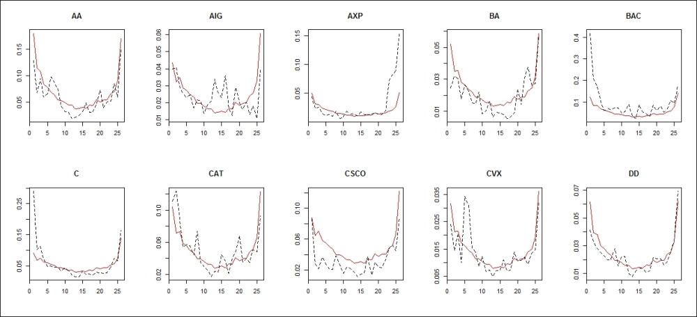
Figure 3.5: Turnover forecasts and realizations for the next day AR(1) is used on the dynamic component

We can conclude that the forecasts appear fairly precise visually. When the realization resembles a more regular U shape, the forecasts can better approximate it (Alcoa, Caterpillar, Chevron, and Du Pont De Nemours), but the one-off large values will always be unpredictable (like the fifth observation in Chevron). The forecasts perform poorly when the realization becomes unusually asymmetric; that is, either the first few or the last few trades are much larger than the rest (American Express, Bank of America, and Citigroup), but even in those cases, the rest of the day is reasonably well approximated.

We can use some code similar to what we used earlier in order to plot the results of the SETAR-based estimation. The output is shown in Figure 3.6.

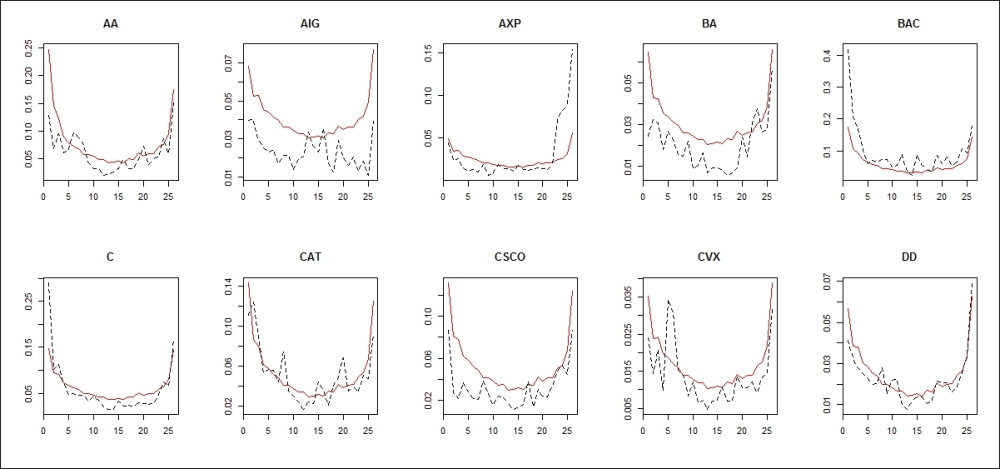
Figure 3.6: Turnover forecasts and realizations for the next day SETAR is used on the dynamic component

At first glance, the results appear very similar to the previous case, which is understandable, because the forecast of the seasonal component is the same in both of them, and apparently, this dominates the forecast; the rest is merely due to individual deviations. The difference between the AR-based and SETAR-based forecasts is more pronounced towards the beginning of the day.

If we observe the first and the last data points of the day in Figures 3.5 and Figure 3.6, we can find a number of stocks (Alcoa, Bank of America, Citigroup, Caterpillar, Cisco, and Du Pont De Nemours) where the forecast for the last point (and mostly throughout the day) is similar, while the forecast for the first point is significantly larger in the case of SETAR. The most noticeable difference between the two forecasts is in the American International and Boeing stocks, where SETAR produces higher values throughout the day.