
How has the DNT price been evolving during the second quarter of 2014? We have the open-high-low-close type time series with five minute frequency for AUDUSD, so we know all the extreme prices:
d <- read.table("audusd.csv", colClasses = c("character", rep("numeric",5)), sep = ";", header = TRUE)
underlying <- as.vector(t(d[, 2:5]))
t <- rep( d[,6], each = 4)
n <- length(t)
option_price <- rep(0, n)

for (i in 1:n) {
  option_price[i] <- dnt1(S = underlying[i], K = 1000000, U = 0.9600, L = 0.9200, sigma = 0.06, T = t[i]/(60*24*365), r = 0.0025, b = -0.0250)
}
a <- min(option_price)
b <- max(option_price)
option_price_transformed = (option_price - a) * 0.03 / (b - a) + 0.92

par(mar = c(6, 3, 3, 5))
matplot(cbind(underlying,option_price_transformed), type = "l",
    lty = 1, col = c("grey", "red"),
    main = "Price of underlying and DNT",
    xaxt = "n", yaxt = "n",  ylim = c(0.91,0.97),
    ylab = "", xlab = "Remaining time")
abline(h = c(0.92, 0.96), col = "green")
axis(side = 2, at = pretty(option_price_transformed),
    col.axis = "grey", col = "grey")
axis(side = 4, at = pretty(option_price_transformed),
    labels = round(seq(a/1000,1000,length = 7)), las = 2,
    col = "red", col.axis = "red")
axis(side = 1, at = seq(1,n, length=6),
    labels = round(t[round(seq(1,n, length=6))]/60/24))
The following is the output for the preceding code:
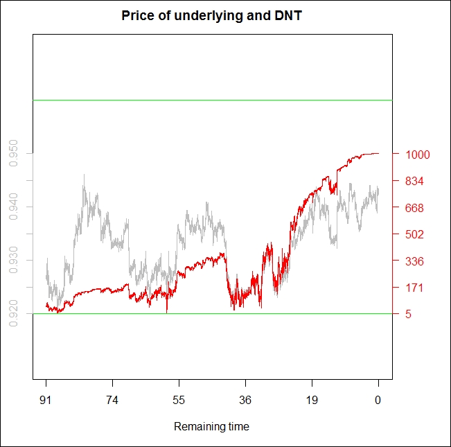
The price of a DNT is shown in red on the right axis (divided by 1000), and the actual AUDUSD price is shown in grey on the left axis. The green lines are the barriers of 0.9200 and 0.9600. The chart shows that in 2014 Q2, the AUDUSD currency pair was traded inside the (0.9200; 0.9600) interval; thus, the payout of the DNT would have been USD 1 million. This DNT looks like a very good investment; however, reality is just one trajectory out of an a priori almost infinite set. It could have happened differently. For example, on May 02, 2014, there were still 59 days left until expiry, and AUDUSD was traded at 0.9203, just three pips away from the lower barrier. At this point, the price of this DNT was only USD 5,302 dollars which is shown in the following code:
dnt1(0.9203, 1000000, 0.9600, 0.9200, 0.06, 59/365, 0.0025, -0.025)
[1] 5302.213
Compare this USD 5,302 to the initial USD 48,564 option price!
In the following simulation, we will show some different trajectories. All of them start from the same 0.9266 AUDUSD spot price as it was on the dawn of April 01, and we will see how many of them stayed inside the (0.9200; 0.9600) interval. To make it simple, we will simulate geometric Brown motions by using the same 6 percent volatility as we used to price the DNT:
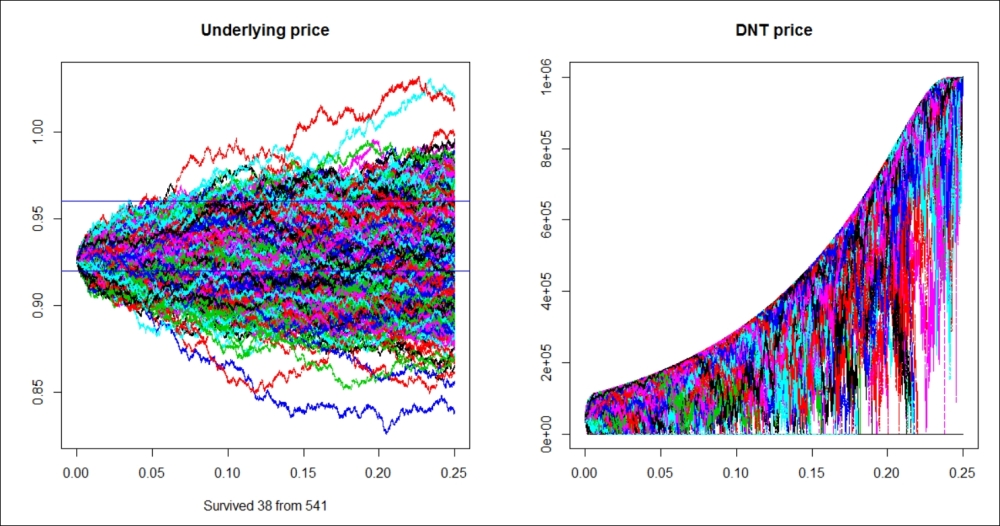
library(matrixStats)
DNT_sim <- function(S0 = 0.9266, mu = 0, sigma = 0.06, U = 0.96,
  L = 0.92, N = 5) {
    dt <- 5 / (365 * 24 * 60)
    t <- seq(0, 0.25, by = dt)
    Time <- length(t)

    W <- matrix(rnorm((Time - 1) * N), Time - 1, N)
    W <- apply(W, 2, cumsum)
    W <- sqrt(dt) * rbind(rep(0, N), W)
    S <- S0 * exp((mu - sigma^2 / 2) * t + sigma * W )
    option_price <- matrix(0, Time, N)

    for (i in 1:N)
       for (j in 1:Time)
          option_price[j,i] <- dnt1(S[j,i], K = 1000000, U, L, sigma,
               0.25-t[j], r = 0.0025,
               b = -0.0250)*(min(S[1:j,i]) > L & max(S[1:j,i]) < U)

    survivals <- sum(option_price[Time,] > 0)
    dev.new(width = 19, height = 10)

    par(mfrow = c(1,2))
    matplot(t,S, type = "l", main = "Underlying price",
        xlab = paste("Survived", survivals, "from", N), ylab = "")
    abline( h = c(U,L), col = "blue")
    matplot(t, option_price, type = "l", main = "DNT price",
        xlab = "", ylab = "")}

set.seed(214)
system.time(DNT_sim())
The following is the output for the preceding code:
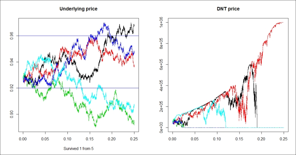
Here, the only surviving trajectory is the red one; in all other cases, the DNT hits either the higher or the lower barrier. The line set.seed(214) grants that this simulation will look the same anytime we run this. One out of five is still not that bad; it would suggest that for an end user or gambler who does no dynamic hedging, this option has an approximate value of 20 percent of the payout (especially since the interest rates are low, the time value of money is not important).
However, five trajectories are still too few to jump to such conclusions. We should check the DNT survivorship ratio for a much higher number of trajectories.
The ratio of the surviving trajectories could be a good estimator of the a priori real-world survivorship probability of this DNT; thus, the end user value of it. Before increasing N rapidly, we should keep in mind how much time this simulation took. For my computer, it took 50.75 seconds for N = 5, and 153.11 seconds for N = 15.
The following is the output for N = 15:
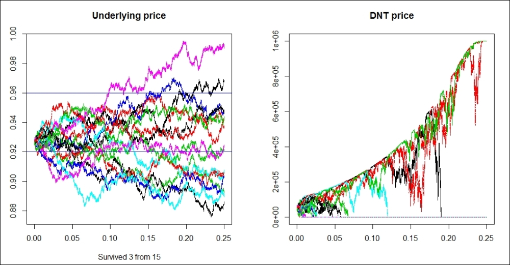
Now, 3 out of 15 survived, so the estimated survivorship ratio is still 3/15, which is equal to 20 percent. Looks like this is a very nice product; the price is around 5 percent of the payout, while 20 percent is the estimated survivorship ratio. Just out of curiosity, run the simulation for N equal to 200. This should take about 30 minutes.
The following is the output for N = 200:
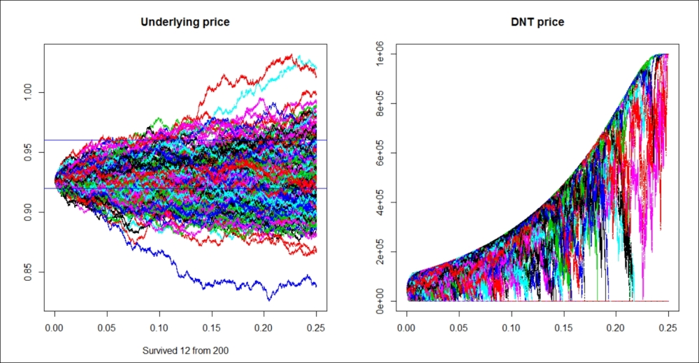
The results are shocking; now, only 12 out of 200 survive, and the ratio is only 6 percent! So to get a better picture, we should run the simulation for a larger N.
The movie Whatever Works by Woody Allen (starring Larry David) is 92 minutes long; in simulation time, that is N = 541. For this N = 541, there are only 38 surviving trajectories, resulting in a survivorship ratio of 7 percent.
What is the real expected survivorship ratio? Is it 20 percent, 6 percent, or 7 percent? We simply don't know at this point. Mathematicians warn us that the law of large numbers requires large numbers, where large is much more than 541, so it would be advisable to run this simulation for as large an N as time allows. Of course, getting a better computer also helps to do more N during the same time. Anyway, from this point of view, Hui's (1996) relatively fast converging DNT pricing formula gets some respect.
So far, we have used the very same stochastic process for pricing that we used for the simulation. Common sense says that in some cases, market-implied volatility could be biased as either higher or lower than the expected volatility. Not surprisingly, running the simulation for these two conditions, N = 200 and sigma = 5.5 percent, results in more surviving trajectories, 15 for this seed. Running the simulation for N = 200 and sigma = 6.5 percent results in fewer surviving trajectories: nine for this seed. This again shows the high impact of vega in a very intuitive way. The number of surviving trajectories, which can be 9, 12, or 15, mostly depends on the volatility of the process. Survivorship rates are 4.5 percent, 6 percent, or 7.5 percent. This also raises a more philosophical question: what about risk premium? If the market needs vega, it could happen that we can purchase a DNT based on 6 percent volatility even if we expect 5.5 percent volatility. In some tense circumstances, the market could be really vega-thirsty. In these cases, risk premium is included.
Derivative pricing always assumes dynamic hedging because we are looking for the marginal cost of producing such an instrument then we use the no-arbitrage argument. Some market players are actually trying to play this strategy and become providers for the derivatives, like a factory. They are willing to take any side of a deal, since they will eliminate almost all of their risks by almost continuous dynamic hedging. They are the market makers. However, not all market players are derivative factories; there are many of them who deliberately seek sensitivities; thus, they are not hedging their derivative position. This second group is called the market takers or end users. Some of them are looking for sensitivities because they already have some and they want to decrease those (natural hedgers). Some others don't have any sensitivities at the beginning, but would like to make a financial bet (speculators).
Interestingly, there could be a significant difference between the price of the derivative and its value for the end user. By purchasing a DNT, an end-user can make a bet and eventually either get nothing, or win much more than the initial price. Is there any risk premium for this bet, or is it similar to a casino? Is the real-life expected value of a DNT higher than the risk-neutral expected value (which equals the price)? The value in use or the "user experience" could be different because the market maker will quote a price based on the implied volatilities. In the case of a tense market situation, the demand for vega could push its price (that is, the implied volatility) higher than the expected volatility.
In this case, anyone who can still sell volatility will get a premium. In the case of DNT, getting a premium means that its price will be lower than the real life expected value of its payout.
What about a Double-one-touch (DOT)? Since the Treasury Bill can be seen as the sum of a DNT and a DOT, if the DNT is too cheap, then the DOT must be too expensive. Thus, these exotic options are easy bets on volatilities; if a speculator thinks volatility will be significantly lower than the implied, purchasing a DNT is a straightforward bet. If the speculator expects higher volatility than the implied, a DOT is the proper bet.
In this sense, DNT is similar to a short straddle and DOT is to a long straddle; however, binary options are much easier to calibrate to the desired size. A long straddle is a long call and long put in the same size, strike price, and expiry. A short straddle is the mirror picture: short call and short put. A strangle is very similar to a straddle; the only difference is that the strike price of a call is not equal but higher than the strike price of the put. Compared to a short straddle or a short strangle, betting on volatility is much more convenient by purchasing a DNT, because holding a long DNT option position requires no further collateral adjustment. DNT is a highly-leveraged product; however, the total amount that can be lost is already paid upfront, so it fits to the menu of online trading platforms where the typical client is a small retail speculator.
Based on this logic, the risk premium goes only to players who are willing to take a position that is less favorable by other market players. If there is an extra demand for volatility, then DNTS will include risk premium, but if there is an extra supply for volatility then DOTs will include risk premium. It could also happen that the market is in a stable equilibrium and neither DNTs nor DOTs include any risk premium.