
Until this point, we considered the entire sample as one. It could be a logical decision to focus only on some industries. Note that choosing the right industry to invest should not be based on past performance pattern; we rather have to analyze comovements with global economic trends over a number of years, and then, based on our prediction for the coming periods, we should pick the one with the best outlook. This method helps you to determine the right weights of the industries in your portfolio, but then, you still need to select individual shares that may overperform the others.
Of course, once one given industry is selected, we may end up with different investment rules than those on the whole sample. So, we may further improve our investment performance by performing the previously shown steps for each industry separately.
At the same time, recall that the more specific you are in data selection (time period, industry, and firm size), the less likely will the strategy created show good performance on other samples or in the future. By increasing the degree of freedom of your strategy building (rerunning all statistical tests for subsamples), you make recommendations fit nearly perfectly to the given sample that may reflect the effects of a number of random events. As these random effects never occur again, adding more and more flexibility after a certain limit will actually worsen the end result.
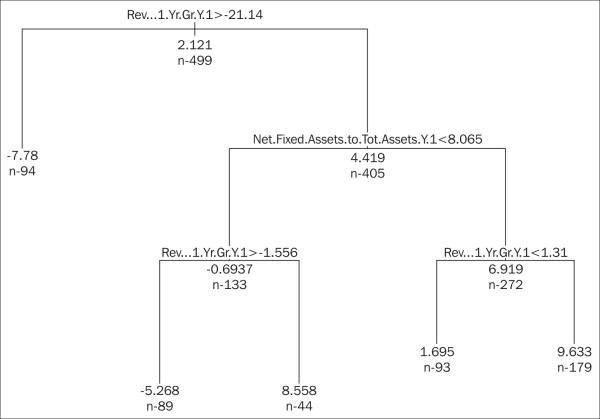
For the sake of the example, we picked Communications. If we apply the decision-tree technique here, we would end up with the following figure. After that, we have to invest into firms that have seen their revenue growing by less than 21 percent but more than 1.31 percent during the last year, while the net fixed assets ratio was at least 8.06 percent:
d_comm <- d[d[,18] == "Communications",c(3:17,19)]
vars <- colnames(d_comm)
m <- length(vars)
tree_formula <- paste(vars[m], paste(vars[-m], collapse = " + "), sep = " ~ ")
library(rpart)
tree <- rpart(formula = tree_formula, data = d_comm, maxdepth = 5 ,cp = 0.01, control = rpart.control(minsplit = 100))
tree <- prune(tree, cp = 0.006)
par(xpd = T)
plot(tree)
text(tree, cex = .5, use.n = T, all = T)
print(tree)
At the same time, building a strategy based on a general sample of a given period may end up overweighting certain industries that show great performance during the given year(s), while, of course, there is no guarantee that the coming years will also prefer the same sectors. So, after building our strategy, we should crosscheck whether there is a serious industry dependency behind that strategy.
A cross-table controlling for the connection of the industry and decision-tree-based investment strategy reveals that we heavily overweighted the Energy and Utilities sectors. The cluster-based strategy, at the same time, gives an extra weight to materials. The code for the latter is shown here:
cross <- table(d[,18], d$selected)
colnames(cross) <- c("not selected", "selected")
cross
                         not selected selected
  Communications                  488       11
  Consumer Discretionary         1476       44
  Consumer Staples                675       36
  Energy                          449       32
  Financials                      116        1
  Health Care                     535       37
  Industrials                    1179       53
  Materials                       762       99
  Technology                      894        7
  Utilities                       287       17

prop.table(cross)

                         not selected     selected
  Communications         0.0677966102 0.0015282023
  Consumer Discretionary 0.2050569603 0.0061128091
  Consumer Staples       0.0937760489 0.0050013893
  Energy                 0.0623784385 0.0044456794
  Financials             0.0161155877 0.0001389275
  Health Care            0.0743262017 0.0051403168
  Industrials            0.1637954987 0.0073631564
  Materials              0.1058627396 0.0137538205
  Technology             0.1242011670 0.0009724924
  Utilities              0.0398721867 0.0023617672
We may also be interested in how good our strategy performs across industries. For this, we should see the average TRS of firms chosen and not chosen for all the individual sectors. To create a table like this, we need to use the following command. The output illustrates how the decision-tree-based strategy performs (0 not selected, 1 selected):
t1 <- aggregate(d[ d$tree,19], list(d[ d$tree,18]), function(x) c(mean(x), median(x)))
t2 <- aggregate(d[!d$tree,19], list(d[!d$tree,18]), function(x) c(mean(x), median(x)))
industry_crosstab <- round(cbind(t1$x, t2$x),4)
colnames(industry_crosstab) <- c("mean-1","median-1","mean-0","median-0")
rownames(industry_crosstab) <- t1[,1]
industry_crosstab

                        mean-1 median-1 mean-0 median-0
Communications         10.4402  11.5531 1.8810   2.8154
Consumer Discretionary 15.9422  10.7034 2.7963   1.3154
Consumer Staples       14.2748   6.5512 4.5523   3.1839
Energy                 17.8265  16.7273 5.6107   5.0800
Financials             33.3632  33.9155 5.4558   3.5193
Health Care            26.6268  21.8815 7.5387   4.6022
Industrials            29.2173  17.6756 6.5487   3.7119
Materials              22.9989  21.3155 8.4270   5.6327
Technology             43.9722  46.8772 7.4596   5.3433
Utilities              11.6620  11.1069 8.6993   7.7672
As shown in the preceding output, our strategy performs pretty well in all sectors; though in Consumer Staples, the median of the selected firms is somewhat near to that of not selected. In other cases, we may end up seeing that in some sectors, we do not get very good results, and the TRS of the chosen firms may even be lower than that of the other group. In this case, we would build a separate stock-selection model for those sectors where our model performed weaker.