Managing interest rate risk is one of the most important components of asset and liability management. Variation of the interest rate could affect both the interest earnings and the market value of equity. Interest rate management focuses on the sensitivity of net interest income. Net interest income (NII) equals the difference between interest revenues and interest expenses:

Here, SA and SL denote the interest sensitive assets and liabilities, and NSA and NSL refer to the non-sensitive ones. Interest rate of assets and liabilities are noted with and . The traditional approach of interest rate risk positioning of the balance sheet is based on gap models. Interest rate gap refers to the net asset position for a certain time period between interest-bearing assets and liabilities, which are repriced at the same time. The interest rate gap (G) equals:

The re-pricing gap table shows these interest-bearing items in the balance sheet grouped by the time of repricing and the basis of repricing (that is, 3 months EURIBOR or 6 months EURIBOR). Interest earnings variation can be characterized as the risk-bearing items multiplied by the change of interest rate (Δi), shown as follows:

The sign of the gap is crucial from an interest rate risk point of view. A positive gap indicates increasing earnings when interest rates rise, and indicates decreasing earnings when interest rates decline. The repricing gap table can also capture the basis risk by aggregating the interest-bearing assets and liabilities based on their reference interest rate (that is 3 months or 6 months EURIBOR). Interest rate gap tables can be sufficient tools to determine the risk exposure from the earnings perspective. However, gap models cannot be used as a single risk measure to quantify rather the net interest income risk of the total balance sheet. Interest rate gaps are management tools, which provide guidance on interest rate risk positioning.

Here, we show how to build up net interest income and repricing gap tables and how to create figures about the net interest income term structure. Let's construct the interest rate gap table from the cashflow.table data. Continuing from the previous section, we use the predefined nii.table function to produce the desired data form:

nii <- nii.table(cashflow.table, now = NOW)

Considering the net interest income table for the next 7 years, we get the following table:

round(nii[,1:7], 2)
           2014    2015    2016    2017    2018   2019   2020
afs_1      6.99    3.42    0.00    0.00    0.00   0.00   0.00
cb_1       0.04    0.00    0.00    0.00    0.00   0.00   0.00
cl_1     134.50  210.04   88.14   29.38    0.89   0.00   0.00
cor_sd_1  -3.20  -11.16   -8.56   -5.96   -3.36  -0.81   0.00
cor_td_1  -5.60   -1.99    0.00    0.00    0.00   0.00   0.00
is_1     -26.17  -80.54  -65.76  -48.61  -22.05  -1.98   0.00
mmp_1      0.41    0.00    0.00    0.00    0.00   0.00   0.00
mmt_1     -0.80   -1.60    0.00    0.00    0.00   0.00   0.00
oth_a_1    0.00    0.00    0.00    0.00    0.00   0.00   0.00
oth_l_1    0.00    0.00    0.00    0.00    0.00   0.00   0.00
rep_1     -0.05    0.00    0.00    0.00    0.00   0.00   0.00
ret_sd_1  -8.18  -30.66  -27.36  -24.06  -20.76 -17.46 -14.16
ret_td_1 -10.07  -13.27    0.00    0.00    0.00   0.00   0.00
rm_1     407.66 1532.32 1364.32 1213.17 1062.75 908.25 751.16
ro_1     137.50  187.50    0.00    0.00    0.00   0.00   0.00
total    633.04 1794.05 1350.78 1163.92 1017.46 888.00 736.99 

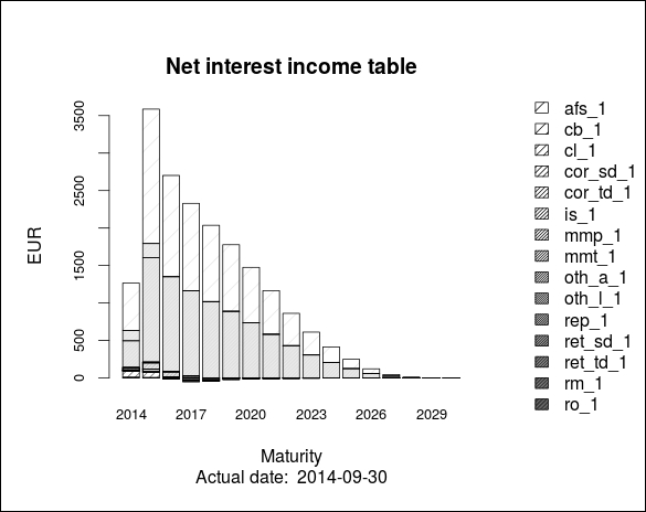
It is easy to read what account brings interest revenues or costs for the bank. The net interest rate table can be plotted as follows:

barplot(nii, density = 5*(1:(NROW(nii)-1)), xlab = "Maturity", cex.names = 0.8, Ylab = "EUR", cex.axis = 0.8, args.legend = list(x = "right"))
title(main = "Net interest income table", cex = 0.8, sub = paste("Actual date: ",as.character(as.Date(NOW))) )par (fig = c(0, 1, 0, 1), oma = c(0, 0, 0, 0),mar = c(0, 0, 0, 0),new = TRUE)
plot(0, 0, type = "n", bty = "n", xaxt = "n", yaxt = "n")
legend("right", legend = row.names(nii[1:(NROW(nii)-1),]), density = 5*(1:(NROW(nii)-1)), bty = "n", cex = 1)

The result is shown in the following graph:

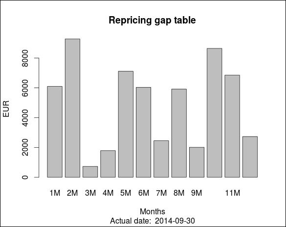
Now, we can explore the re-pricing gaps by composing the re-pricing gap table. Let's use the predefined repricing.gap.table function and get the monthly gaps, and then plot the results with barplot.

(repgap <- repricing.gap.table(portfolio, now = NOW))
         1M   2M  3M   4M   5M   6M   7M   8M   9M  10M  11M  12M
volume 6100 9283 725 1787 7115 6031 2450 5919 2009 8649 6855 2730
barplot(repgap, col = "gray", xlab = "Months", ylab = "EUR")
title(main = "Repricing gap table", cex = 0.8, sub = paste("Actual date: ",as.character(as.Date(NOW))))

With the preceding code, we can illustrate the marginal gaps for the next 12 months:

We have to mention that there are more sophisticated tools for interest rate risk management. In practice, simulation models are applied for risk management purposes. However, the banking book risks are not explicitly subjected to capital charge under Pillar 1 of the Basel II regulations; Pillar 2 covers the interest rate risk in the banking book. Regulators lay particular emphasis also on the risk assessment regarding the market value of equity. Risk limits are based on specific stress scenarios, which could be either deterministic interest rate shocks or historical volatility-based earnings at risk concepts. Therefore, risk measurement techniques stand for scenario-based or stochastic simulation approaches, focusing on the interest earnings or the market value of equity. Net interest income simulation is rather a dynamic, forward-looking approach, while calculation of the market value of equity provides a static result. Equity duration is also a widely used measure for interest rate risk of the banking book. Duration of the assets and liabilities are calculated to quantify the duration of equity. ALM professionals often use effective duration, which incorporates embedded options (caps, floors, and so on) in the interest rate sensitivity calculation.