In the following code, we use Austrian non-maturity deposit time series data that we queried from the ECB Statistical Database, which is publicly available. We have monthly deposit interest rates (cpn), end-of-month balances (bal), and the 1 month EURIBOR fixing (eur1m) in our dataset. The time series are stored in a csv file in the local folder. The command for that is ads follows:

nmd <- read.csv("ecb_nmd_data.csv")
nmd$date <- as.Date(nmd$date, format = "%m/%d/%Y")

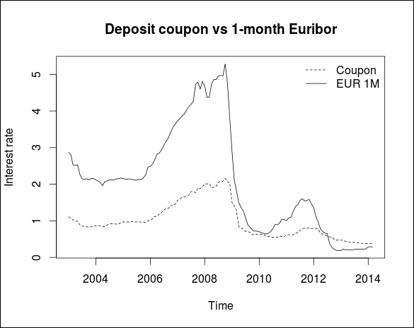
First, we plot the 1 month EURIBOR rate and the deposit interest rate development by using the following command:

library(car)
plot(nmd$eur1m ~ nmd$date, type = "l", xlab="Time", ylab="Interest rate")
lines(nmd$cpn~ nmd$date, type = "l", lty = 2)
title(main = "Deposit coupon vs 1-month Euribor", cex = 0.8 )
legend("topright", legend = c("Coupon","EUR 1M"), bty = "n", cex = 1, lty = c(2, 1))

The following screenshot displays the graph of Deposit Coupon vs 1-month EURIBOR:

Our first goal is to estimate an error correction model (ECM) to describe the long-term explanatory power of 1 month EURIBOR rate on the non-maturity deposit interest rate. Measuring the pass-through effect of market rates into deposit interest rates has gained high importance in recent years from the regulatory point of view as well. ECB required euro-zone banks to estimate the pass-through effect in certain stress-test scenarios. We use the Engle-Granger two-step method to estimate the ECM model. In the first step, we estimate the cointegrating vector with a regression model. We take the residuals, and in the second step, we estimate the long-term and short-term effects of EURIBOR on deposit rates using the error-correction mechanism. Before the first step, we have to test whether both time series are integrated in the same order. Therefore, we run Augmented Dickey-Fuller (ADF) and the KPSS tests from the urca package on the original and the differentiated time series. The script is as follows:

library(urca)
attach(nmd)
#Unit root test (ADF)
cpn.ur <- ur.df(cpn, type = "none", lags = 2)
dcpn.ur <- ur.df(diff(cpn), type = "none", lags = 1)
eur1m.ur <- ur.df(eur1m, type = "none", lags = 2)
deur1m.ur <- ur.df(diff(eur1m), type = "none", lags = 1)
sumtbl <- matrix(cbind(cpn.ur@teststat, cpn.ur@cval,
                       dcpn.ur@teststat, dcpn.ur@cval,
                       eur1m.ur@teststat, eur1m.ur@cval,
                       deur1m.ur@teststat, deur1m.ur@cval), nrow=4)
colnames(sumtbl) <- c("cpn", "diff(cpn)", "eur1m", "diff(eur1m)")
rownames(sumtbl) <- c("Test stat", "1pct CV", "5pct CV", "10pct CV")
#Stationarty test (KPSS)
cpn.kpss <- ur.kpss(cpn, type = "mu")
eur1m.kpss <- ur.kpss(eur1m, type = "mu")
sumtbl <- matrix(cbind( cpn.kpss@teststat, cpn.kpss@cval, eur1m.kpss@teststat, eur1m.kpss@cval), nrow = 5)
colnames(sumtbl) <- c("cpn", "eur1m")
rownames(sumtbl) <- c("Test stat", "10pct CV", "5pct CV", "2.5pct CV", 1pct CV")
print([email protected])
print(sumtbl)
print([email protected])
print(sumtbl)

As a result, we get the following summary tables:

Augmented Dickey-Fuller Test

                 cpn diff(cpn)     eur1m diff(eur1m)
Test stat -0.9001186 -5.304858 -1.045604    -5.08421
1pct CV   -2.5800000 -2.580000 -2.580000    -2.58000
5pct CV   -1.9500000 -1.950000 -1.950000    -1.95000
10pct CV  -1.6200000 -1.620000 -1.620000    -1.62000

KPSS

                cpn    eur1m
Test stat 0.8982425 1.197022
10pct CV  0.3470000 0.347000
5pct CV   0.4630000 0.463000
2.5pct CV 0.5740000 0.574000
1pct CV   0.7390000 0.739000

The null-hypothesis of the ADF test cannot be refused for the original time series, but the test results show that the first difference of the deposit rate and 1 month EURIBOR time series does not contain the unit root. This means that both series are integrated at the first order, and they are I(1) processes. The KPSS test has a similar result. The next step is to test the cointegration of the two I(1) series by testing the residuals of the simple regression equation, where we regress the deposit interest rates on the 1 month EURIBOR rate. Estimate the cointegrating equation:

lr <- lm(cpn ~ eur1m)
res <- resid(lr)
lr$coefficients
(Intercept)       eur1m 
  0.3016268   0.3346139

Do the unit root test of residuals as follows:

res.ur <- ur.df(res, type = "none", lags = 1)
summary(res.ur)
############################################### 
# Augmented Dickey-Fuller Test Unit Root Test # 
############################################### 

Test regression none 

Call:
lm(formula = z.diff ~ z.lag.1 - 1 + z.diff.lag)

Residuals:
      Min        1Q    Median        3Q       Max 
-0.286780 -0.017483 -0.002932  0.019516  0.305720 

Coefficients:
           Estimate Std. Error t value Pr(>|t|)   
z.lag.1    -0.14598    0.04662  -3.131  0.00215 **
z.diff.lag -0.06351    0.08637  -0.735  0.46344   
---
Signif. codes:  0 '***' 0.001 '**' 0.01 '*' 0.05 '.' 0.1 ' ' 1

Residual standard error: 0.05952 on 131 degrees of freedom
Multiple R-squared:  0.08618,   Adjusted R-squared:  0.07223 
F-statistic: 6.177 on 2 and 131 DF,  p-value: 0.002731

Value of test-statistic is: -3.1312 

Critical values for test statistics:
      1pct  5pct 10pct
tau1 -2.58 -1.95 -1.62

The test statistic of the ADF test is lower than the 1 percent critical value, so we can conclude that the residuals are stationary. This means that the deposit coupon and 1 month EURIBOR are cointegrated, as the linear combination of the two I(1) time series gives us a stationary process. The existence of cointegration is important because it is a prerequisite for the error-correction model estimation. The basic structure of an ECM equation is as follows:

We estimate the long-term and short-term effect of X on Y; the lagged residuals from the cointegration equation represent the error-correction mechanism. The coefficient measures the short-term correction part, while is the coefficient of the long-term equilibrium relationship, which captures the correction of deviations from the equilibrium of X. Now, we estimate the ECM model using the dynlm package, which is suitable to estimate dynamic linear models with lags:

install.packages('dynlm')
library(dynlm)
res <- resid(lr)[2:length(cpn)]
dy <- diff(cpn)
dx <- diff(eur1m)
detach(nmd)
ecmdata <- c(dy, dx, res)
ecm <- dynlm(dy ~ L(dx, 1) + L(res, 1), data = ecmdata)
summary(ecm)

Time series regression with "numeric" data:
Start = 1, End = 134

Call:
dynlm(formula = dy ~ L(dx, 1) + L(res, 1), data = ecmdata)

Residuals:
     Min       1Q   Median       3Q      Max 
-0.36721 -0.01546  0.00227  0.02196  0.16999 

Coefficients:
              Estimate Std. Error t value Pr(>|t|)    
(Intercept) -0.0005722  0.0051367  -0.111    0.911    
L(dx, 1)     0.2570385  0.0337574   7.614 4.66e-12 ***
L(res, 1)    0.0715194  0.0534729   1.337    0.183    
---
Signif. codes:  0 '***' 0.001 '**' 0.01 '*' 0.05 '.' 0.1 ' ' 1

Residual standard error: 0.05903 on 131 degrees of freedom
Multiple R-squared:  0.347,	Adjusted R-squared:  0.337 
F-statistic:  34.8 on 2 and 131 DF,  p-value: 7.564e-13

The lagged changes in 1 month EURIBOR are corrected in the deposit interest rates by 25.7 percent () on the short run. We cannot conclude that deviations from the long-term equilibrium are not corrected as beta2 is not significant and has a positive sign, meaning that the errors are not corrected but boosted by 7 percent. The economic interpretation of the results is that we cannot identify a long-term relationship between NMD coupons and 1 month EURIBOR rate, but deviations in the EURIBOR are reflected in the coupons by 25.7 percent in the short term.

A possible method to hedge interest-rate-related risks of non-maturity deposits is to construct a replicating portfolio of zero-coupon instruments to mimic the interest payment of non-maturity deposits, and earn a margin on the higher-yielding replicating instruments over the low interest on deposit accounts.

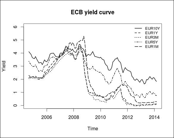
Let's assume that we include 1-month and 3-month EUR money market placements and 1Y, 5Y, and 10Y government benchmark bonds in our replicating portfolio. We queried the historical time series of the yields from ECB Statistical Data Warehouse and stored the data in a csv file in the local folder. We will call the csv file using the following command:

ecb.yc <- read.csv("ecb_yc_data.csv")
ecb.yc$date <- as.Date(ecb.yc$date, format = "%d/%m/%Y")

Plot the results:

matplot(ecb.yc$date, ecb.yc[,2:6], type = "l", lty = (1:5), lwd = 2, col = 1, xlab = "Time", ylab = "Yield", ylim = c(0,6), xaxt = "n")
legend("topright", cex = 0.8, bty = "n", lty = c(1:5), lwd = 2, legend = colnames(ecb.yc[,2:6])) 
title(main = "ECB yield curve", cex = 0.8)
axis.Date(1,ecb.yc$date)

The following screenshot shows the ECB yield curve:

Our goal is to calculate those portfolio weights of the five hedging instruments in the replicating portfolio, which ensures that the minimum volatility of the margin compared to the deposit coupon (cpn) in the given time horizon. In other words, we would like to minimize the tracking error of the interest earning of our replicating portfolio. The problem can be formulated in the following least squares minimization formula:

This is subject to:

Here, A is the matrix's historical rates, b is the vector of the deposit coupons, and x is the vector of portfolio weights. The function to be minimized is the squared difference between the vector b and the linear combination of x with the columns of matrix A. The first condition is that the portfolio weights have to be non-negative and summed up to 1. We introduce an additional condition on the average maturity of the portfolio, which should be equal to the l constant. The vector m contains the maturity in months of the five hedging instruments. The rationale behind this constraint is that banks usually assume that the core base of non-maturity deposit volume stays in the bank for a longer term. The tenor of this long-term part is usually derived from a volume model, which could be the ARIMA model or a dynamic model with dependency on market rates and the deposit coupon.

To solve the optimization problem, we use the solve.QP function from the quadprog package. This function is suitable to solve quadratic optimization problems with equality and inequality constraints. We reformulate the least squares minimization problem in order to derive the proper parameter matrix (A'A) and parameter vector (b'A) of the solve.QP function.

We also set , assuming 5 year final maturity for the replicating portfolio, which mimics the liquidity characteristics of the core part of the NMD portfolio through the following command:

library(quadprog)
b <- nmd$cpn[21:135]
A <- cbind(ecb.yc$EUR1M, ecb.yc$EUR3M, ecb.yc$EUR1Y, ecb.yc$EUR5Y, ecb.yc$EUR10Y)
m <- c(1, 3, 12, 60, 120)
l <- 60
stat.opt <- solve.QP( t(A) %*% A, t(b) %*% A, cbind( matrix(1, nr = 5, nc = 1), matrix(m, nr = 5, nc = 1), diag(5)), c(1, l, 0,0,0,0,0), meq=2 )
sumtbl <- matrix(round(stat.opt$solution*100, digits = 1), nr = 1)
colnames(sumtbl) <- c("1M", "3M", "1Y", "5Y", "10Y")
cat("Portfolio weights in %")
Portfolio weights in % > print(sumtbl)
     1M   3M 1Y 5Y  10Y
[1,]  0 51.3  0  0 48.7

Our result suggests that based on historical calibration, we should keep 51 percent in 3 month money market placement and 49 percent in a 10 year government bond instrument in our replicating portfolio to replicate the coupon development of NMDs with the smallest tracking error. With these portfolio weights, the income on our replicating portfolio and the expense on deposit accounts are calculated by the following code:

mrg <- nmd$cpn[21:135] - stat.opt$solution[2]*ecb.yc$EUR3M + stat.opt$solution[5]*ecb.yc$EUR10Y
plot(mrg ~ ecb.yc$date, type = "l", col = "black", xlab="Time", ylab="%")
title(main = "Margin of static replication", cex = 0.8 )

The following graph displays Margin of static replication:

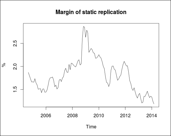
As you can see, due to the replication with this static strategy, a bank was able to earn more profit around 2010, when the term spread between the short- and long-term interest rates was unusually high.