
Banks face various kinds of risks, for example, client default, changes in the market environment, troubles in refinancing, and fraud. These risks are categorized into credit risk, market risk, and operational risk.
Losses realized from the movements of the market prices are covered by the market risk. It may include the losses on the trading book positions of a bank or financial institution, but the losses realized on interest rate or currency that may be in connection with the core business of a bank also belong to market risk. Market risk can include several subcategories such as equity risk, interest rate risk, currency risk, and commodity risk. Liquidity risk is also covered in this topic. Based on the advanced approach of the Basel II directive, the capital needed to cover these risks is mostly based on value at risk calculations.
Currency risk refers to the possible loss on the movements of the foreign exchange rates (for example, EUR/USD) or on its derivative products, while commodity risk covers the losses on the movements of commodity prices (for example, gold, crude oil, wheat, copper, and so on). Currency risk can also affect the core business of a bank if there is a mismatch between the FX exposure in funding and lending. FX mismatch can lead to a serious risk in a bank; thus, regulators usually have strict limitations on the maximum amount of the so-called open FX positions. This results in a mismatch of the FX exposure between the liability and the asset side of the bank. This can be tackled by certain hedging deals (such as cross-currency swaps, currency futures, forwards, FX options, and so on).
Equity risk is the possible loss on stocks, stock indices, or derivative products with equity underlying. We saw examples on how to measure the equity risk using either the standard deviation or the value at risk. Now, we will show examples on how the risk of the equity derivative portfolio can be measured using the already mentioned techniques. First, we look at a single call option's value at risk, and we then analyze how a portfolio of a call and a put option can be dealt by this method.
First, let's assume that all the conditions of the Black-Scholes model consist of the market. For more information on the Black-Scholes model and its condition, refer to the book of John. C. Hull [9]. A stock is currently traded at S = USD 100, which pays no dividend and follows a geometric Brownian motion with μ equal to 20 percent (drift) and σ equal to 30 percent (volatility) parameters.
An ATM (at-the-money) call option on this stock matures in two years from now, and we would like to determine the 95 percent one year value at risk of this option. We know that the stock price follows a lognormal distribution, while the logarithmic rate of return follows a normal distribution with the following m and s parameters:
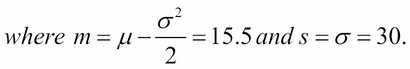
Now, let's calculate the current price of the derivative given that the Black-Scholes conditions exist. Using the Black-Scholes formula, the two-year option is trading at USD 25.98:
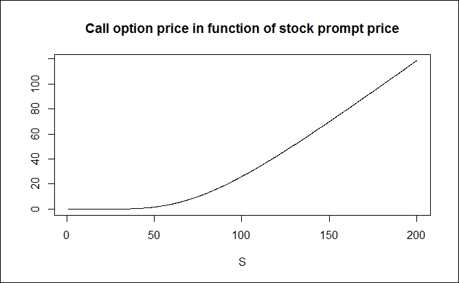
Note that the price of the call option is a monotone-growing function of the spot price of the underlying.
This characteristic helps us a lot in solving this problem. What we need is a threshold of the option price below which it goes with only a 5-percent probability. However, because it is a monotone growing function of S, we only need to know where this threshold is for the stock price. Given the m and s parameters, we can easily find this value using the following formula:
Therefore, we now know that there is only a 5 percent chance that the stock price goes below USD 71.29 in one year (the time period for m and s parameters is one year). If we apply the Black-Scholes formula on this price and with a one year less maturity of the option, we get the threshold for the call option price.
Now, we know that there is a 95 percent likelihood that the option price goes above USD 2.90 in one year. So the value that we lose at most with 95 percent probability is the difference between the actual option price and the threshold. So the call option's 95 percent VaR for one year is as follows:
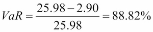
Therefore, the call option on the given stock may only lose more than USD 23.08 or 88.82 percent with 5 percent probability in one year.
The calculations can be seen below in the following R codes. Note that before running the code, we need to install the fOptions library using this command:
install.packages("fOptions")
library(fOptions)

X <- 100
Time <- 2
r <- 0.1
sigma <- 0.3
mu <- 0.2
S <- seq(1,200, length = 1000)
call_price <- sapply(S, function(S) GBSOption("c", S, X, Time, r, r, sigma)@price)
plot(S, call_price, type = "l", ylab = "", main = "Call option price in function of stock prompt price")
The following screenshot is the result of the preceding command:
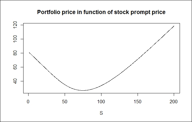
The situation is not that simple if we would like to find the value at risk of a certain portfolio of call and put options. Let's use the previous example with the stock trading at USD 100. Now, we add an ATM put option to the portfolio besides the ATM call option to form a complex position known as straddle in finance. From our point of view, the problem with this portfolio is the non-monotonicity of the function of the stock price. As seen in the chart shown in the next image, the value of this portfolio as a function of the stock price is a parabola or is similar to a V if the option is just before its maturity.
Therefore, the previous logic of finding the appropriate stock price threshold to calculate the option price threshold does not work here. However, we can call the Monte-Carlo simulation method to derive the desired value.
First, let's use the so-called put-call parity to gather the put option's value using the call price that has been calculated previously. The put-call parity is calculated as follows:
Here, c and p is the call and put option prices, both with a strike price of X, and S is the actual stock price Hull (2002). The value of the full portfolio is USD 33.82 as a consequence.
Now, we use the simulation to gather 10,000 realizations of a possible portfolio value derived from a randomly generated set of input data. We ensure that the stock follows a geometric Brownian motion and that the logarithmic rate of return follows a normal distribution with the m and s parameters (15.5 percent and 30 percent). Applying the generated logarithmic return on the original stock price (USD 100), we will reach a simulated stock price for 1 year from now. This can be used to recalculate the value of both the call and put options using the Black-Scholes formula. Note that here, we replace the original stock price with the simulated one, while we also use a one year less maturity for the calculations. As the last step, we create 10,000 realizations of the simulated portfolio value (c + p), and then find the lower fifth percentile. This will be the threshold below which the option portfolio value goes only in 5 percent of the cases. The steps can be seen in the following code:
X <- 100
Time <- 2
r <- 0.1
sigma <- 0.3
mu <- 0.2
S <- seq(1,200, length = 1000)
call_price <- sapply(S, function(S) GBSOption("c", S, X, Time, r, r, sigma)@price)
put_price <- sapply(S, function(S) GBSOption("p", S, X, Time, r, r, sigma)@price)
portfolio_price <- call_price + put_price
windows()
plot(S, portfolio_price, type = "l", ylab = "", main = "Portfolio price in function of stock prompt price")
# portfolio VaR simulation
p0 <- GBSOption("c", 100, X, Time, r, r, sigma)@price + GBSOption("p", 100, X, Time, r, r, sigma)@price
print(paste("price of portfolio:",p0))
[1] "price of portfolio: 33.8240537586255"
S1 <- 100*exp(rnorm(10000, mu - sigma^2 / 2 , sigma))
P1 <- sapply(S1, function(S) GxBSOption("c", S, X, 1, r, r, sigma)@price + GBSOption("p", S, X, 1, r, r, sigma)@price )
VaR <- quantile(P1, 0.05)
print(paste("95% VaR of portfolio: ", p0 - VaR))
The preceding command yields the following output:
The desired threshold came out at USD 21.45; thus, the value at risk of the portfolio is 33.82 - 21.45 = USD 12.37. Therefore, the probability that the portfolio loses more than 12.37 in one year is only 5 percent.
Interest rate risk arises from the core business, that is, the lending and refinancing activity of a bank. However, it also includes the possible losses on bonds or fixed income derivatives due to unfavorable changes in interest rates. The interest rate risk is the most important market risk for a bank, given the fact that it mostly uses short-term funding (client deposits, interbank loans, and so on) to refinance long-term assets (such as mortgage loans, government bonds, and so on).
Calculating the value at risk of a position or the whole portfolio can be a useful tool to measure the market risk of a bank or financial institution. However, several other tools are also available to measure and to cope with the interest rate risk for example. Such a tool can be the analysis of the mismatch of the interest-sensitivity gap between assets and liabilities. This method was among the first techniques in asset liability management to measure and tackle interest-rate risk, but it is much less accurate than the modern risk measurement methods. In the interest-sensitivity gap analysis, asset and liability elements are classified by the average maturity or the timing of interest-rate reset in case the asset or liability is a floater. Then, the asset and liability elements are compared in each time period class to give a detailed view on the interest-rate sensitivity mismatch.
The VaR-based approach is a much more developed and accurate measure for the interest rate risk of a bank or financial institution. This method is also based on the interest rate sensitivity and is represented by the duration (and convexity) of a fixed income portfolio rather than the maturity mismatch of asset and liability elements.
The primary risk that a bank faces is the possible default of the borrower, where the required payment is failed to be made. Here, the risk is that the lender loses the principal, the interest, and all related payments. The loss can be partial or complete depending on the collateral and other mitigating factors. The default can be a consequence of a number of different circumstances such as payment failure from a retail borrower on mortgage, a credit card, or a personal loan; the insolvency of a company, bank, or insurance firm; a failed payment on an invoice due; the failure of payment by the issuer on debt securities, and so on.
The expected loss from credit risk can be represented as a multiple of three different factors: the PD, LGD, and EAD:
Probability of default (PD) is the likelihood that the event of failed payment happens. This is the key factor of all credit risk models, and there are several types of approaches to estimate this value. The loss given default (LGD) is the proportion that is lost in percentage of the claimed par value. The recovery rate (RR) is the inverse of LGD and shows the amount that can be collected (recovered) even if the borrower defaults. This is affected by the collaterals and other mitigating factors used in lending. The exposure at the default (EAD) is the claimed value that is exposed to the certain credit risk.
Banks and financial institutions use different methods to measure and handle credit risk. In order to reduce it, all the three factors of the multiple can be in focus. To keep the exposure under control, banks may use limits and restrictions in lending towards certain groups of clients (consumers, companies, and sovereigns). Loss given default can be lowered by using collaterals such as mortgage rights on properties, securities, and guarantees. Collaterals provide security to the lenders and ensure that they get back at least some of their money. Other tools are also available to reduce loss given default, such as credit derivatives and credit insurance.
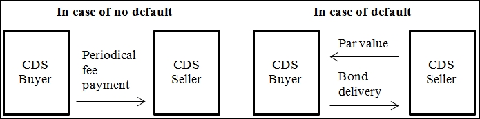
A credit default swap (CDS) is a financial swap agreement that works as insurance against the default of a third party. The issuer or seller of the CDS agrees to compensate the buyer in an event that the debt holder defaults. The buyer pays a periodical fee for the seller set in percentage of the par value of the bond or other debt security. The seller pays the par value to the buyer and receives the bond in the case of a credit event. If there is no default by the debtor, the CDS deal terminates at maturity without any payment from the seller.
The probability of default can be mitigated by due diligence of the business partners and the borrowers, using covenants and strict policies. Banks use a broad variety of due diligence, ranging from the standardized scoring processes to more complex in-depth research on clients. By applying these methods, banks can screen out those clients who have too high probability of default and would therefore hit the capital position. Credit risk can also be mitigated by risk-based pricing. Higher probability of default leads to a higher expected loss on credit risk that has to be covered by the interest rate spread applied to the specific client. Banks need to tackle this in their normal course of business and only need to form capital to the unexpected loss. Therefore, the expected loss on credit risk should be a basic part of product pricing.
Estimating the probability of default is a very important issue for all banks and financial institutions. There are several approaches, of which we examine three different ones:
- An implicit probability is derived from the market pricing of risky bonds or credit default swaps (for example, the Hull-White method)
- Structural models (for example, the KMV model)
- Current and historic movements of credit ratings (for example, CreditMetrics)
The first approach assumes that there are traded products on the market related to the instruments as an underlying that have credit risk. It is also assumed that the risk is perfectly shown in the market pricing of such instruments. For example, if a bond of a risky company is traded on the market, the price of the bond will be lower than the price of a risk-free security. If a credit default swap is traded on the market on a certain bond, then, it also reflects the market's evaluation of the risk on that security. If there is enough liquidity on the market, the expected credit risk loss should be equal to the observed price of the risk. If we know this price, we can determine the implicit probability of the default price.
Let's take a look at a short example. Let's assume that a 1 year maturity zero-coupon bond with a par value of USD 1,000 issued by a BBB-rated corporation trades at a YTM (yield-to-maturity) of 5 percent. An AAA-rated government T-Bill with similar characteristics but without credit risk trades at 3 percent. We know that if the corporate bond defaults, 30 percent of the par value will be recovered. What is the probability of the bond defaulting if the market prices properly?
First, we need to calculate the current market price of both the corporate and the government bond. The corporate bond should trade at 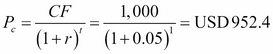 . Similarly, the government bond should trade at
 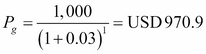 .
.
The price difference between the two bonds is USD 18.5. The expected credit loss is PD∙LGD∙EAD in one year. If we wanted to take a hedge against the credit loss through insurance or CDS, the present value of this amount would be the maximum that we would pay. As a consequence, the price difference of the two bonds should equal to the present value of the expected credit loss. The LGD is 70 percent as 30 percent of the par value is recovered in the case of a default.
Therefore, ![]() or
or ![]() .
.
So the implicit probability of default is 2.72 percent during the next year, if the market prices are proper. This method can also be used if there is a credit derivative traded on the market related to the specific bond.
Structural methods create a mathematical model based on the characteristics of the financial instrument that is exposed to the credit risk. A common example is the KMV model created by the joint company founded by three mathematicians, Stephen Kealhofer, John McQuown, and Oldřich Vašíček. Currently, this company runs under the name of Moody's Analytics after having been acquired by Moody's rating agency in 2002.
The KMV model is based on Merton's credit model (1974), which regards both the debt and equity securities of a corporation with credit risk as derivatives similar to options. The basic idea is that if a company is solvent, then the market value of its assets (or enterprise value) should exceed the par value of the debts it holds. Therefore, just before the maturity of the corporate bonds, they estimate their par value and the value of the equity (market capitalization of a public company). However, if the value of assets misses the par value of debt at maturity, the owners might decide to raise the capital or go bankrupt. If the latter is the case, the market value of corporate bonds will equal the asset value, and the equity holders will get nothing during liquidation.
The choice between the bankruptcy and capital raising is called the bankruptcy option, which has the characteristics of a put option. This exists because the equity holders have no more responsibility on the company than the value they invested (the share price cannot go to negative). More specifically, the value of the corporate bond is the combination of a bond without credit risk and a bankruptcy option, which is a short put option from the point of view of the bondholder (long bond + short put).
The equity of the company can be treated as a call option (long call). The asset value of the company is the sum of all the equations, as shown in this formula: ![]() , where D is the par value of the corporate debt, V is the asset value, c is the market value of the equity (the call option in this regard), and p is the value of the bankruptcy option.
, where D is the par value of the corporate debt, V is the asset value, c is the market value of the equity (the call option in this regard), and p is the value of the bankruptcy option.
The KMV model
In practice, the volatility of both the asset value and the equity is necessary to calculate the actual value of the risky corporate bond. A public company's equity volatility can easily be estimated from stock price movements, but the asset volatility is not available as real economy goods are usually not traded publicly. The market value of assets is also a tricky one due to the same reason. Therefore, the KMV has two equations and two unknown variables. The two equations are the conditions of the Black-Scholes theory ![]() , which is based on the Black-Scholes equation, and
, which is based on the Black-Scholes equation, and ![]() , which is based on Itō's lemma, where E and V are the market values of equity and assets, D is the par value of the bond, σE and σV are the volatilities of the equity and the assets. The
, which is based on Itō's lemma, where E and V are the market values of equity and assets, D is the par value of the bond, σE and σV are the volatilities of the equity and the assets. The ![]() is the derivative of E with respect to V, and it equals to N(d1), based on the Black-Scholes theory. The two unknown variables are V and σV.
is the derivative of E with respect to V, and it equals to N(d1), based on the Black-Scholes theory. The two unknown variables are V and σV.
Now, let's take a look at an example where the market value of a company's equity (market capitalization) is USD 3 billion with 80 percent volatility. The company has a single series of zero-coupon bonds with a par value of USD 10 billion, which matures exactly in one year. The risk-free logarithmic rate of return is 5 percent for one year.
The solution of the preceding equation in R can be seen as follows:
install.packages("fOptions")
library(fOptions)
kmv_error <- function(V_and_vol_V, E=3,Time=1,D=10,vol_E=0.8,r=0.05){
  V <- V_and_vol_V[1]
  vol_V <- V_and_vol_V[2]
  E_ <- GBSOption("c", V, D, Time, r, r, vol_V)@price
  tmp <- vol_V*sqrt(Time)
  d1 <- log(V/(D*exp(-r*Time)))/tmp + tmp/2
  Nd1 <- pnorm(d1)
  vol_E_ <- Nd1*V/E*vol_V
  err <- c(E_ - E, vol_E_ - vol_E)
  err[1]^2+err[2]^2
}
a <- optim(c(1,1), fn = kmv_error)
print(a)
The value of the aggregate of the corporate bonds is USD 9.40 billion with a logarithmic of yield to maturity at 6.44 percent, and the value of the assets are USD 12.40 billion with 21.2 percent volatility.
The third way of estimating the probability of default is the rating-based approach. This method of estimation starts from the credit rating of different financial instruments or economic entities (companies, sovereigns, and institutions). CreditMetrics analytics was originally developed by JP Morgan's risk management division in 1997. Since then, it has evolved further, and now, it is widely used among other risk management tools. The basic idea of CreditMetrics is to estimate probabilities on how the credit rating of an entity can change over time and what effect it can have on the value of the securities issued by the same entity. It starts with the analysis of the rating history and then creates a so-called transition matrix that contains the probabilities of how the credit rating might develop. For further information on CreditMetrics, see the technical book published by MSCI (Committee on Banking Regulations and Supervisory Practices (1987)).
The third major risk category is the operational risk. This refers to all the possible losses that can arise during the operation of a bank, financial institution, or another company. It includes losses from natural disasters, internal or external fraud (for example, bank robbery), system faults or failures, and inadequate working processes. These risks can be categorized into four different groups seen below:
- Low impact with low probability: If the risk as well as its potential impact on the operation is low, then it is not worth the effort to handle it.
- Low impact with high probability: If a risk event happens too often, it means that some processes of the company should be restructured, or it should be included in the pricing of a certain operation.
- High impact with low probability: If the probability of a high-impact event is low, the most suitable method to mitigate the risk is to take insurance on such events.
- High impact with high probability: If both the impact and the probability of such a risk are high, then it's better to shut down that operation. Here, neither the restructuring nor the insurance works.
This part of the risk management belongs rather to the actuarial sciences than financial analysis. However, the tools provided by R are also capable of handling such problems as well. Let's take an example of the possible operational losses on the failures of an IT system. The number of failures follow a Poisson distribution with λ = 20 parameter, while the magnitude of each loss follows a lognormal distribution with m equal to 5 and s equal to 2 parameters. The average number of failures in a year is 20 based on the Poisson distribution, while the expected value of the magnitude of a loss is: ![]() .
.
However, we need to determine the joint distribution, the expected value, and the quantile of 99.9 percent of the aggregate annual loss. The latter will be used to determine the necessary capital set by the advanced measurement approach (AMA) of Basel II. We use a 10,000 element Monte-Carlo simulation. The first step is to generate a discrete random variable that follows a Poisson distribution. Then, we generate independent variables with lognormal distribution in the number of the previously generated integers, and we aggregate them. We can create the distribution of the aggregated losses by repeating this process 10,000 times. The expected value of the aggregate losses is USD 21,694, and the quantile of 99.9 percent is USD 382,247.
Therefore, we will only lose more than USD 382 thousand in a year by the failure of the IT system in 0.1 percent of the cases. The calculations can be seen in R here:
op <- function(){
n <- rpois(1, 20)
z <- rlnorm(n,5,2)
sum(z)
}
Loss <- replicate(10000, op())
hist(Loss[Loss<50000], main = "", breaks = 20, xlab = "", ylab = "")
print(paste("Expected loss = ", mean(Loss)))
print(paste("99.9% quantile of loss = ", quantile(Loss, 0.999)))
The following is the screenshot of the preceding command:
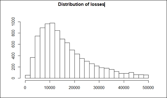
We see the distribution of the aggregated losses in the chart shown in the preceding figure, which is similar to a lognormal distribution but is not necessarily lognormal.