Elastic net regularization is a method that reduces the danger of overfitting in the context of regression (see http://en.wikipedia.org/wiki/Elastic_net_regularization). The elastic net regularization combines linearly the least absolute shrinkage and selection operator (LASSO) and ridge methods. LASSO limits the so-called L1 norm or Manhattan distance. This norm measures for a points pair the sum of absolute coordinates differences. The ridge method uses a penalty, which is the L1 norm squared. For regression problems, the goodness-of-fit is often determined with the coefficient of determination also called R squared (see http://en.wikipedia.org/wiki/Coefficient_of_determination). Unfortunately, there are several definitions of R squared. Also, the name is a bit misleading, since negative values are possible. A perfect fit would have a coefficient of determination of one. Since the definitions allow for a wide range of acceptable values, we should aim for a score that is as close to one as possible.

Let's use a 10-fold cross-validation. Define an ElasticNetCV object, as follows:

clf = ElasticNetCV(max_iter=200, cv=10, l1_ratio = [.1, .5, .7, .9, .95, .99, 1])

The ElasticNetCV class has an l1_ratio argument with values between 0 and 1. If the value is 0, we have only ridge regression; if it is one, we have only LASSO regression. Otherwise, we have a mixture. We can either specify a single number or a list of numbers to choose from. For the rain data, we get the following score:

Score 0.0527838760942

This score suggests that we are underfitting the data. This can occur for several reasons, such as we are not using enough features or the model is wrong. For the Boston house price data, with all the present features we get:

Score 0.683143903455

The predict() method gives prediction for new data. We will visualize the quality of the predictions with a scatter plot. For the rain data, we obtain the following plot:

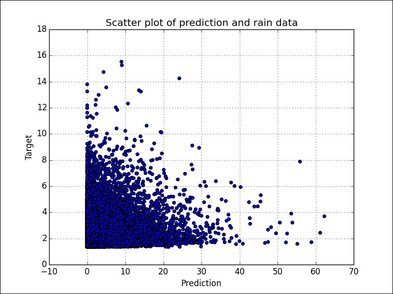
The plot in the previous figure confirms that we have a bad fit (underfitting). A straight diagonal line through the origin would indicate a perfect fit. That's almost what we get for the Boston house price data:

Refer to the encv.py file in this book's code bundle:

from sklearn.linear_model import ElasticNetCV
import numpy as np
from sklearn import datasets
import matplotlib.pyplot as plt


def regress(x, y, title):
    clf = ElasticNetCV(max_iter=200, cv=10, l1_ratio = [.1, .5, .7, .9, .95, .99, 1])

    clf.fit(x, y)
    print "Score", clf.score(x, y)

    pred = clf.predict(x)
    plt.title("Scatter plot of prediction and " + title)
    plt.xlabel("Prediction")
    plt.ylabel("Target")
    plt.scatter(y, pred)
    # Show perfect fit line
    if "Boston" in title:
        plt.plot(y, y, label="Perfect Fit")
        plt.legend()

    plt.grid(True)
    plt.show()

rain = .1 * np.load('rain.npy')
rain[rain < 0] = .05/2
dates = np.load('doy.npy')

x = np.vstack((dates[:-1], rain[:-1]))
y = rain[1:]
regress(x.T, y, "rain data")

boston = datasets.load_boston()
x = boston.data
y = boston.target
regress(x, y, "Boston house prices")