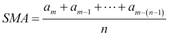
Moving averages are frequently used to analyze time series. A moving average specifies a window of data that is previously seen, which is averaged each time the window slides forward by one period:

The different types of moving averages differ essentially in the weights used for averaging. The exponential moving average, for instance, has exponentially decreasing weights with time:

This means that older values have less influence than newer values, which is sometimes desirable.

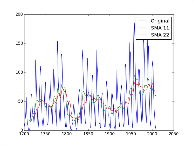
The following code from the moving_average.py file in this book's code bundle plots the simple moving average for the 11- and 22-year sunspots cycles:

import matplotlib.pyplot as plt
import statsmodels.api as sm
from pandas.stats.moments import rolling_mean

data_loader = sm.datasets.sunspots.load_pandas()
df = data_loader.data
year_range = df["YEAR"].values
plt.plot(year_range, df["SUNACTIVITY"].values, label="Original")
plt.plot(year_range, rolling_mean(df, 11)["SUNACTIVITY"].values, label="SMA 11")
plt.plot(year_range, rolling_mean(df, 22)["SUNACTIVITY"].values, label="SMA 22")
plt.legend()
plt.show()

We can express an exponential decreasing weight strategy for the exponential moving average, as shown in the following NumPy code:

weights = np.exp(np.linspace(-1., 0., N))
weights /= weights.sum()

A simple moving average uses equal weights, which in code looks as follows:

def sma(arr, n):
   weights = np.ones(n) / n

   return np.convolve(weights, arr)[n-1:-n+1] 

Since we can load the data into a pandas DataFrame, it is more convenient to use the pandas rolling_mean() function. Load the data as follows using statsmodels:

data_loader = sm.datasets.sunspots.load_pandas()
df = data_loader.data

Refer to the following plot for the end result: