Profiling is about identifying parts of the code that are slow or use a lot of memory. We will profile a modified version of the sentiment.py code from Chapter 9, Analyzing Textual Data and Social Media. The code is refactored to comply with multiprocessing programming guidelines. You will learn about multiprocessing later in this chapter. Also, we simplified the stopwords filtering. The third change is to have fewer word features as the reduction doesn't impact accuracy. This last change has the most impact. The original code ran for about 20 seconds. The new code runs faster than that and will serve as the baseline in this chapter. Some changes have to do with profiling and will be explained later in this section. Please refer to the prof_demo.py file in this book's code bundle:

import random
from nltk.corpus import movie_reviews
from nltk.corpus import stopwords
from nltk import FreqDist
from nltk import NaiveBayesClassifier
from nltk.classify import accuracy
from lprof_hack import profile

@profile
def label_docs():
    docs = [(list(movie_reviews.words(fid)), cat)
            for cat in movie_reviews.categories()
            for fid in movie_reviews.fileids(cat)]
    random.seed(42)
    random.shuffle(docs)

    return docs

@profile
def isStopWord(word):
    return word in sw or len(word) == 1

@profile
def filter_corpus():
    review_words = movie_reviews.words()
    print "# Review Words", len(review_words)
    res = [w.lower() for w in review_words if not isStopWord(w.lower())]
    print "# After filter", len(res)

    return res
@profile
def select_word_features(corpus):
    words = FreqDist(corpus)
    N = int(.02 * len(words.keys()))
    return words.keys()[:N]

@profile
def doc_features(doc):
    doc_words = FreqDist(w for w in doc if not isStopWord(w))
    features = {}
    for word in word_features:
        features['count (%s)' % word] = (doc_words.get(word, 0))
    return features

@profile
def make_features(docs):
    return [(doc_features(d), c) for (d,c) in docs]

@profile
def split_data(sets):
    return sets[200:], sets[:200]

if __name__ == "__main__":
    labeled_docs = label_docs()

    sw = set(stopwords.words('english'))
    filtered = filter_corpus()
    word_features = select_word_features(filtered)
    featuresets = make_features(labeled_docs)
    train_set, test_set = split_data(featuresets)
    classifier = NaiveBayesClassifier.train(train_set)
    print "Accuracy", accuracy(classifier, test_set)
    print classifier.show_most_informative_features()

When we measure time, it helps to have as few processes running as possible. However, we can't be sure that nothing is running in the background, so we will take the lowest time measured from three measurements with the time command. This is a command available on various operating systems and Cygwin. Run the command as follows:

$ time python prof_demo.py

We get a real time, which is the time we would measure using a clock. The user and sys times measure the CPU time used by the program. The sys time is the time spent in the kernel. On my machine, the following times in seconds were obtained (the lowest values were placed between brackets):

Profile the code with the standard Python profiler as follows:

$ python -m cProfile -o /tmp/stat.prof prof_demo.py

The –o switch specifies an output file. We can visualize the profiler output with the gprof2dot PyPi package. Install it as follows:

$ pip install gprof2dot
$ pip freeze|grep gprof2dot
gprof2dot==2014.08.05

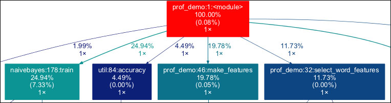
Create a PNG visualization with the following command:

$ gprof2dot -f pstats /tmp/stat.prof |dot -Tpng -o /tmp/cprof.png

The full image is too large to display here; here is a small excerpt of it:

Query the profiler output as follows:

$ python -m pstats /tmp/stat.prof

With this command, we enter the profile statistics browser. Strip the filenames from the output, sort by time, and show the top 10 times:

/tmp/stat.prof% strip
/tmp/stat.prof% sort time
/tmp/stat.prof% stats 10

Refer to the following screenshot for the end result:

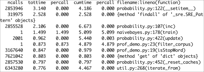
The following is a description of the headers:

The line_profiler is another profiler we can use. This profiler is still in beta, but it can display statistics for each line in functions, which have been decorated with the @profile decorator. Also, it requires a workaround, which has been included in the lprof_hack.py file in this book's code bundle. The workaround is from an Internet forum (refer to https://stackoverflow.com/questions/18229628/python-profiling-using-line-profiler-clever-way-to-remove-profile-statements). Install and run this profiler with the following commands:

$ pip install --pre line_profiler
$ kernprof.py -l -v prof_demo.py

The full report is too long to reproduce here; instead, the following is a per-function summary (there is some overlap):

Function: label_docs at line 9 Total time: 6.19904 s
Function: isStopWord at line 19 Total time: 2.16542 s
File: prof_demo.py Function: filter_corpus at line 23
Function: select_word_features at line 32 Total time: 4.05266 s
Function: doc_features at line 38 Total time: 12.5919 s
Function: make_features at line 46 Total time: 14.566 s
Function: split_data at line 50 Total time: 3.6e-05 s