Multiprocessing is a standard Python module that targets machines with multiple processors. Multiprocessing works around the Global Interpreter Lock (GIL) by creating multiple processes.

Multiprocessing supports process pools, queues, and pipes. A process pool is a pool of system processes that can execute a function in parallel. Queues are data structures that are usually used to store tasks. Pipes connect different processes in such a way that the output of one process becomes the input of another.

Create a pool and register a function as follows:

   p = mp.Pool(nprocs)

The pool has a map() method that is the parallel equivalent of the Python map() function:

p.map(simulate, [i for i in xrange(10, 50)])

We will simulate the movement of a particle in one dimension. The particle performs a random walk and we are interested in computing the average end position of the particle. We repeat this simulation for different walk lengths. The calculation itself is not important. The important part is to compare the speedup with multiple processes versus a single process. We will plot the speedup with matplotlib. The full code is in the multiprocessing_sim.py file in this book's code bundle:

from numpy.random import random_integers
from numpy.random import randn
import numpy as np
import timeit
import argparse
import multiprocessing as mp
import matplotlib.pyplot as plt


def simulate(size):
    n = 0
    mean = 0
    M2 = 0

    speed = randn(10000)

    for i in xrange(1000): 
        n = n + 1
        indices = random_integers(0, len(speed)-1, size=size)
        x = (1 + speed[indices]).prod()
        delta = x - mean
        mean = mean + delta/n
        M2 = M2 + delta*(x - mean)

    return mean

def serial():
    start = timeit.default_timer()

    for i in xrange(10, 50):
        simulate(i)

    end = timeit.default_timer() - start
    print "Serial time", end

    return end
def parallel(nprocs):
    start = timeit.default_timer()
    p = mp.Pool(nprocs)
    print nprocs, "Pool creation time", timeit.default_timer() - start

    p.map(simulate, [i for i in xrange(10, 50)])
    p.close()
    p.join()

    end = timeit.default_timer() - start
    print nprocs, "Parallel time", end
    return end

if __name__ == "__main__":
    ratios = []
    baseline = serial()

    for i in xrange(1, mp.cpu_count()):
        ratios.append(baseline/parallel(i))

    plt.xlabel('# processes')
    plt.ylabel('Serial/Parallel')
    plt.plot(np.arange(1, mp.cpu_count()), ratios)
    plt.grid(True)
    plt.show()

If we take the speedup values for process pool sizes ranging from 1 to 8 (the number of processors is hardware dependent), we get the following figure:

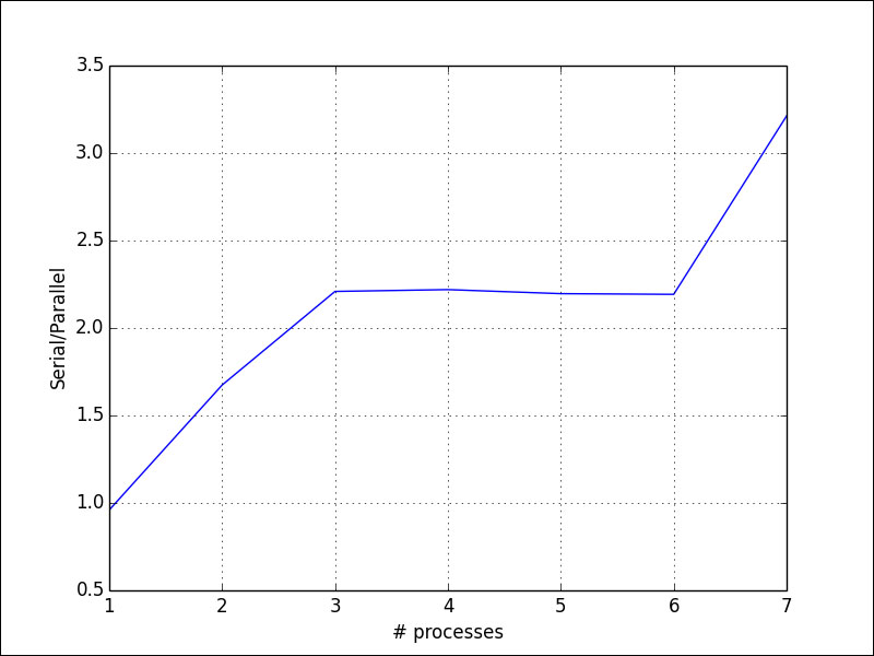
Amdahl's law (see http://en.wikipedia.org/wiki/Amdahl%27s_law) best describes the speedups due to parallelization. This law predicts the maximum possible speedup. The number of processes limits the absolute maximum speedup. However, as we can see in the preceding plot, we don't get a doubling of speed with two processes nor does using three processes triple the speed, but we come close. Some parts of any given Python code may be impossible to parallelize. For example, we may need to wait for a resource to become available or we may be performing a calculation that has to be performed sequentially. We also have to take into account overhead from parallelization setup and related interprocess communication. Amdahl's law states that there is a linear relationship between the inverse of the speedup, the inverse of the number of processes, and the portion of the code, which cannot be parallelized.