
We have already learned about the reshape() function. Another repeating chore is the flattening of arrays. Flattening in this setting entails transforming a multidimensional array into a one-dimensional array. The code for this example is in the shapemanipulation.py file in this book's code bundle.
import numpy as np

# Demonstrates multi dimensional arrays slicing.
#
# Run from the commandline with
#
#  python shapemanipulation.py
print "In: b = arange(24).reshape(2,3,4)"
b = np.arange(24).reshape(2,3,4)

print "In: b"
print b
#Out:
#array([[[ 0,  1,  2,  3],
#        [ 4,  5,  6,  7],
#        [ 8,  9, 10, 11]],
#
#       [[12, 13, 14, 15],
#        [16, 17, 18, 19],
#        [20, 21, 22, 23]]])

print "In: b.ravel()"
print b.ravel()
#Out:
#array([ 0,  1,  2,  3,  4,  5,  6,  7,  8,  9, 10, 11, 12, 13, 14, 15, 16,
#       17, 18, 19, 20, 21, 22, 23])

print "In: b.flatten()"
print b.flatten()
#Out:
#array([ 0,  1,  2,  3,  4,  5,  6,  7,  8,  9, 10, 11, 12, 13, 14, 15, 16,
#       17, 18, 19, 20, 21, 22, 23])

print "In: b.shape = (6,4)"
b.shape = (6,4)

print "In: b"
print b
#Out:
#array([[ 0,  1,  2,  3],
#       [ 4,  5,  6,  7],
#       [ 8,  9, 10, 11],
#       [12, 13, 14, 15],
#       [16, 17, 18, 19],
#       [20, 21, 22, 23]])

print "In: b.transpose()"
print b.transpose()
#Out:
#array([[ 0,  4,  8, 12, 16, 20],
#       [ 1,  5,  9, 13, 17, 21],
#       [ 2,  6, 10, 14, 18, 22],
#       [ 3,  7, 11, 15, 19, 23]])


print "In: b.resize((2,12))"
b.resize((2,12))

print "In: b"
print b
#Out:
#array([[ 0,  1,  2,  3,  4,  5,  6,  7,  8,  9, 10, 11],
#       [12, 13, 14, 15, 16, 17, 18, 19, 20, 21, 22, 23]])
We can manipulate array shapes using the following functions:
- Ravel: We can accomplish this with the
ravel()function as follows:In: b Out: array([[[ 0, 1, 2, 3], [ 4, 5, 6, 7], [ 8, 9, 10, 11]], [[12, 13, 14, 15], [16, 17, 18, 19], [20, 21, 22, 23]]]) In: b.ravel() Out: array([ 0, 1, 2, 3, 4, 5, 6, 7, 8, 9, 10, 11, 12, 13, 14, 15, 16, 17, 18, 19, 20, 21, 22, 23]) - Flatten: The appropriately named function,
flatten(), does the same asravel(). However,flatten()always allocates new memory, whereasravelmight give back a view of the array. This means that we can directly manipulate the array as follows:In: b.flatten() Out: array([ 0, 1, 2, 3, 4, 5, 6, 7, 8, 9, 10, 11, 12, 13, 14, 15, 16, 17, 18, 19, 20, 21, 22, 23]) - Setting the shape with a tuple: Besides the
reshape()function, we can also define the shape straightaway with a tuple, which is exhibited as follows:In: b.shape = (6,4) In: b Out: array([[ 0, 1, 2, 3], [ 4, 5, 6, 7], [ 8, 9, 10, 11], [12, 13, 14, 15], [16, 17, 18, 19], [20, 21, 22, 23]])As you can understand, the preceding code alters the array immediately. Now, we have a 6 x 4 array.
- Transpose: In linear algebra, it is common to transpose matrices. Transposing is a way to transform data. For a two-dimensional table, transposing means that rows become columns and columns become rows. We can do this too by using the following code:
In: b.transpose() Out: array([[ 0, 4, 8, 12, 16, 20], [ 1, 5, 9, 13, 17, 21], [ 2, 6, 10, 14, 18, 22], [ 3, 7, 11, 15, 19, 23]]) - Resize: The
resize()method works just like thereshape()method, but changes the array it works on:In: b.resize((2,12)) In: b Out: array([[ 0, 1, 2, 3, 4, 5, 6, 7, 8, 9, 10, 11], [12, 13, 14, 15, 16, 17, 18, 19, 20, 21, 22, 23]])
Arrays can be stacked horizontally, depth wise, or vertically. We can use, for this goal, the vstack(), dstack(), hstack(), column_stack(), row_stack(), and concatenate() functions. To start with, let's set up some arrays (refer to stacking.py in this book's code bundle):
In: a = arange(9).reshape(3,3)
In: a
Out:
array([[0, 1, 2],
       [3, 4, 5],
       [6, 7, 8]])
In: b = 2 * a
In: b
Out:
array([[ 0,  2,  4],
       [ 6,  8, 10],
       [12, 14, 16]])
As mentioned previously, we can stack arrays using the following techniques:
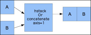
- Horizontal stacking: Beginning with horizontal stacking, we will shape a tuple of
ndarraysand hand it to thehstack()function to stack the arrays. This is shown as follows:In: hstack((a, b)) Out: array([[ 0, 1, 2, 0, 2, 4], [ 3, 4, 5, 6, 8, 10], [ 6, 7, 8, 12, 14, 16]])We can attain the same thing with the
concatenate()function, which is shown as follows:In: concatenate((a, b), axis=1) Out: array([[ 0, 1, 2, 0, 2, 4], [ 3, 4, 5, 6, 8, 10], [ 6, 7, 8, 12, 14, 16]])The following diagram depicts horizontal stacking:
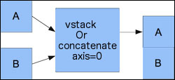
- Vertical stacking: With vertical stacking, a tuple is formed again. This time it is given to the
vstack()function to stack the arrays. This can be seen as follows:In: vstack((a, b)) Out: array([[ 0, 1, 2], [ 3, 4, 5], [ 6, 7, 8], [ 0, 2, 4], [ 6, 8, 10], [12, 14, 16]])The
concatenate()function gives the same outcome with the axis parameter fixed to0. This is the default value for the axis parameter, as portrayed in the following code:In: concatenate((a, b), axis=0) Out: array([[ 0, 1, 2], [ 3, 4, 5], [ 6, 7, 8], [ 0, 2, 4], [ 6, 8, 10], [12, 14, 16]])Refer to the following figure for vertical stacking:
- Depth stacking: To boot, there is the depth-wise stacking employing
dstack()and a tuple, of course. This entails stacking a list of arrays along the third axis (depth). For example, we could stack 2D arrays of image data on top of each other as follows:In: dstack((a, b)) Out: array([[[ 0, 0], [ 1, 2], [ 2, 4]], [[ 3, 6], [ 4, 8], [ 5, 10]], [[ 6, 12], [ 7, 14], [ 8, 16]]]) - Column stacking: The
column_stack()function stacks 1D arrays column-wise. This is shown as follows:In: oned = arange(2) In: oned Out: array([0, 1]) In: twice_oned = 2 * oned In: twice_oned Out: array([0, 2]) In: column_stack((oned, twice_oned)) Out: array([[0, 0], [1, 2]])2D arrays are stacked the way the
hstack()function stacks them, as demonstrated in the following lines of code:In: column_stack((a, b)) Out: array([[ 0, 1, 2, 0, 2, 4], [ 3, 4, 5, 6, 8, 10], [ 6, 7, 8, 12, 14, 16]]) In: column_stack((a, b)) == hstack((a, b)) Out: array([[ True, True, True, True, True, True], [ True, True, True, True, True, True], [ True, True, True, True, True, True]], dtype=bool)Yes, you guessed it right! We compared two arrays with the
==operator. - Row stacking: NumPy, naturally, also has a function that does row-wise stacking. It is named
row_stack()and for 1D arrays, it just stacks the arrays in rows into a 2D array:In: row_stack((oned, twice_oned)) Out: array([[0, 1], [0, 2]])The
row_stack()function results for 2D arrays are equal to thevstack()function results:In: row_stack((a, b)) Out: array([[ 0, 1, 2], [ 3, 4, 5], [ 6, 7, 8], [ 0, 2, 4], [ 6, 8, 10], [12, 14, 16]]) In: row_stack((a,b)) == vstack((a, b)) Out: array([[ True, True, True], [ True, True, True], [ True, True, True], [ True, True, True], [ True, True, True], [ True, True, True]], dtype=bool)
Arrays can be split vertically, horizontally, or depth wise. The functions involved are
hsplit(), vsplit(), dsplit(), and split(). We can split arrays either into arrays of the same shape or indicate the location after which the split should happen. Let's look at each of the functions in detail:
- Horizontal splitting: The following code splits a 3 x 3 array on its horizontal axis into three parts of the same size and shape (see
splitting.pyin this book's code bundle):In: a Out: array([[0, 1, 2], [3, 4, 5], [6, 7, 8]]) In: hsplit(a, 3) Out: [array([[0], [3], [6]]), array([[1], [4], [7]]), array([[2], [5], [8]])]Liken it with a call of the
split()function, with an additional argument,axis=1:In: split(a, 3, axis=1) Out: [array([[0], [3], [6]]), array([[1], [4], [7]]), array([[2], [5], [8]])] - Vertical splitting:
vsplit()splits along the vertical axis:In: vsplit(a, 3) Out: [array([[0, 1, 2]]), array([[3, 4, 5]]), array([[6, 7, 8]])]
The
split()function, withaxis=0, also splits along the vertical axis:In: split(a, 3, axis=0) Out: [array([[0, 1, 2]]), array([[3, 4, 5]]), array([[6, 7, 8]])]
- Depth-wise splitting: The
dsplit()function, unsurprisingly, splits depth-wise. We will require an array of rank3to begin with:In: c = arange(27).reshape(3, 3, 3) In: c Out: array([[[ 0, 1, 2], [ 3, 4, 5], [ 6, 7, 8]], [[ 9, 10, 11], [12, 13, 14], [15, 16, 17]], [[18, 19, 20], [21, 22, 23], [24, 25, 26]]]) In: dsplit(c, 3) Out: [array([[[ 0], [ 3], [ 6]], [[ 9], [12], [15]], [[18], [21], [24]]]), array([[[ 1], [ 4], [ 7]], [[10], [13], [16]], [[19], [22], [25]]]), array([[[ 2], [ 5], [ 8]], [[11], [14], [17]], [[20], [23], [26]]])]
Let's learn more about the NumPy array attributes with the help of an example. For this example, see arrayattributes2.py provided in the book's code bundle:
import numpy as np

# Demonstrates ndarray attributes.
#
# Run from the commandline with
#
#  python arrayattributes2.py
b = np.arange(24).reshape(2, 12)
print "In: b"
print b
#Out:
#array([[ 0,  1,  2,  3,  4,  5,  6,  7,  8,  9, 10, 11],
#       [12, 13, 14, 15, 16, 17, 18, 19, 20, 21, 22, 23]])

print "In: b.ndim"
print b.ndim
#Out: 2

print "In: b.size"
print b.size
#Out: 24

print "In: b.itemsize"
print b.itemsize
#Out: 8

print "In: b.nbytes"
print b.nbytes
#Out: 192

print "In: b.size * b.itemsize"
print b.size * b.itemsize
#Out: 192

print "In: b.resize(6,4)"
print b.resize(6,4)

print "In: b"
print b
#Out:
#array([[ 0,  1,  2,  3],
#       [ 4,  5,  6,  7],
#       [ 8,  9, 10, 11],
#       [12, 13, 14, 15],
#       [16, 17, 18, 19],
#       [20, 21, 22, 23]])

print "In: b.T"
print b.T
#Out:
#array([[ 0,  4,  8, 12, 16, 20],
#       [ 1,  5,  9, 13, 17, 21],
#       [ 2,  6, 10, 14, 18, 22],
#       [ 3,  7, 11, 15, 19, 23]])

print "In: b.ndim"
print b.ndim
#Out: 1

print "In: b.T"
print b.T
#Out: array([0, 1, 2, 3, 4])


print "In: b = array([1.j + 1, 2.j + 3])"
b = np.array([1.j + 1, 2.j + 3])

print "In: b"
print b
#Out: array([ 1.+1.j,  3.+2.j])

print "In: b.real"
print b.real
#Out: array([ 1.,  3.])

print "In: b.imag"
print b.imag
#Out: array([ 1.,  2.])

print "In: b.dtype"
print b.dtype
#Out: dtype('complex128')

print "In: b.dtype.str"
print b.dtype.str
#Out: '<c16'


print "In: b = arange(4).reshape(2,2)"
b = np.arange(4).reshape(2,2)

print "In: b"
print b
#Out:
#array([[0, 1],
#       [2, 3]])

print "In: f = b.flat"
f = b.flat

print "In: f"
print f
#Out: <numpy.flatiter object at 0x103013e00>

print "In: for it in f: print it"
for it in f:
   print it
#0
#1
#2
#3

print "In: b.flat[2]"
print b.flat[2]
#Out: 2


print "In: b.flat[[1,3]]"
print b.flat[[1,3]]
#Out: array([1, 3])


print "In: b"
print b
#Out:
#array([[7, 7],
#       [7, 7]])

print "In: b.flat[[1,3]] = 1"
b.flat[[1,3]] = 1

print "In: b"
print b
#Out:
#array([[7, 1],
#       [7, 1]])
Besides the shape and dtype attributes, ndarray has a number of other properties, as shown in the following list:
ndimgives the number of dimensions, as shown in the following code snippet:In: b Out: array([[ 0, 1, 2, 3, 4, 5, 6, 7, 8, 9, 10, 11], [12, 13, 14, 15, 16, 17, 18, 19, 20, 21, 22, 23]]) In: b.ndim Out: 2sizeholds the count of elements. This is shown as follows:In: b.size Out: 24
itemsizereturns the count of bytes for each element in the array, as shown in the following code snippet:In: b.itemsize Out: 8
- If you require the full count of bytes the array needs, you can have a look at
nbytes. This is just a product of theitemsizeandsizeproperties:In: b.nbytes Out: 192 In: b.size * b.itemsize Out: 192
- The
Tproperty has the same result as thetranspose()function, which is shown as follows:In: b.resize(6,4) In: b Out: array([[ 0, 1, 2, 3], [ 4, 5, 6, 7], [ 8, 9, 10, 11], [12, 13, 14, 15], [16, 17, 18, 19], [20, 21, 22, 23]]) In: b.T Out: array([[ 0, 4, 8, 12, 16, 20], [ 1, 5, 9, 13, 17, 21], [ 2, 6, 10, 14, 18, 22], [ 3, 7, 11, 15, 19, 23]]) - If the array has a rank of less than 2, we will just get a view of the array:
In: b.ndim
Out: 1
In: b.T
Out: array([0, 1, 2, 3, 4])
- Complex numbers in NumPy are represented by
j. For instance, we can produce an array with complex numbers as follows:In: b = array([1.j + 1, 2.j + 3]) In: b Out: array([ 1.+1.j, 3.+2.j])
- The
realproperty returns to us the real part of the array, or the array itself if it only holds real numbers:In: b.real Out: array([ 1., 3.])
- The
imagproperty holds the imaginary part of the array:In: b.imag Out: array([ 1., 2.])
- If the array holds complex numbers, then the data type will automatically be complex as well:
In: b.dtype Out: dtype('complex128') In: b.dtype.str Out: '<c16' - The
flatproperty gives back anumpy.flatiterobject. This is the only means to get aflatiterobject; we do not have access to aflatiterconstructor. Theflatiterator enables us to loop through an array as if it were a flat array, as shown in the following code snippet:In: b = arange(4).reshape(2,2) In: b Out: array([[0, 1], [2, 3]]) In: f = b.flat In: f Out: <numpy.flatiter object at 0x103013e00> In: for item in f: print item .....: 0 1 2 3It is possible to straightaway obtain an element with the
flatiterobject:In: b.flat[2] Out: 2
Also, you can obtain multiple elements as follows:
In: b.flat[[1,3]]
Out: array([1, 3])
The
flatproperty can be set. Setting the value of theflatproperty leads to overwriting the values of the entire array:In: b.flat = 7 In: b Out: array([[7, 7], [7, 7]])We can also obtain selected elements as follows:
In: b.flat[[1,3]] = 1
In: b
Out:
array([[7, 1],
       [7, 1]])
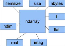
The next diagram illustrates various properties of ndarray:
We can convert a NumPy array to a Python list with the
tolist() function (refer to arrayconversion.py in this book's code bundle). The following is a brief explanation:
- Convert to a list:
In: b
Out: array([ 1.+1.j,  3.+2.j])
In: b.tolist()
Out: [(1+1j), (3+2j)]
- The
astype()function transforms the array to an array of the specified data type:In: b Out: array([ 1.+1.j, 3.+2.j]) In: b.astype(int) /usr/local/bin/ipython:1: ComplexWarning: Casting complex values to real discards the imaginary part #!/usr/bin/python Out: array([1, 3]) In: b.astype('complex') Out: array([ 1.+1.j, 3.+2.j])
The preceding code won't display a warning this time because we used the right data type.