As mentioned before, support vector machines can be used for regression. In the case of regression, we are using a hyperplane not to separate points, but for a fit. A learning curve is a way to visualize the behavior of a learning algorithm. It is a plot of training and test scores for a range of train data sizes. Creating a learning curve forces us to train the estimator multiple times and is therefore on aggregate slow. We can compensate for this by creating multiple concurrent estimator jobs. Support vector regression is one of the algorithms that may require scaling. We get the following top scores:

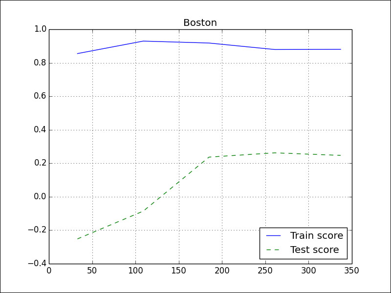
Max test score Rain 0.0161004084576
Max test score Boston 0.662188537037

This is similar to the results obtained with the ElasticNetCV class. Many scikit-learn classes have an n_jobs parameter for that purpose. As a rule of thumb, we often create as many jobs as there are CPUs in our system. The jobs are created using the standard Python multiprocessing API. Call the learning_curve() function to perform training and testing:

train_sizes, train_scores, test_scores = learning_curve(clf, X, Y, n_jobs=ncpus)

Plot scores by averaging them:

plt.plot(train_sizes, train_scores.mean(axis=1), label="Train score")
plt.plot(train_sizes, test_scores.mean(axis=1), '--', label="Test score")

The rain data learning curve looks like this:

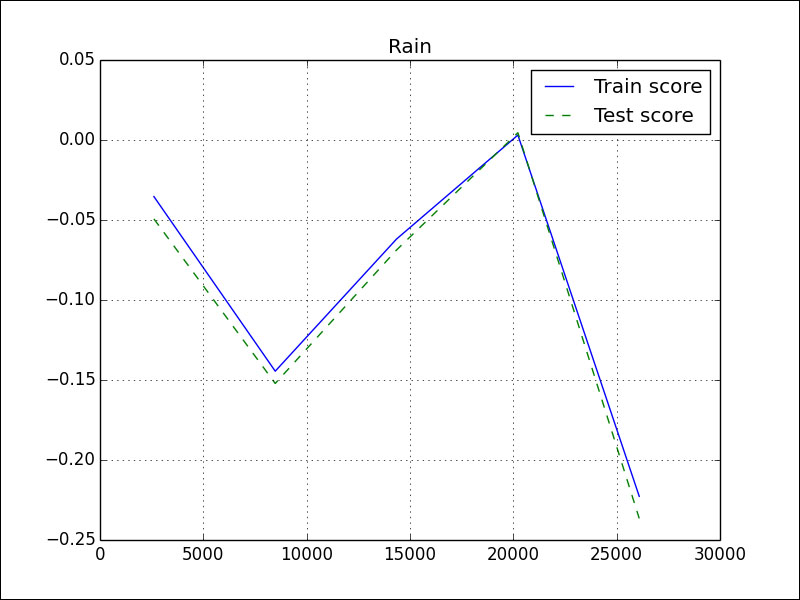
A learning curve is something we are familiar with in our daily lives. The more experience we have, the more we should have learned. In data analysis terms, we should have a better score if we add more data. If we have a good training score, but a poor test score, this means that we are overfitting. Our model only works on the training data. The Boston house price data learning curve looks much better:

The code is in the sv_regress.py file in this book's code bundle:

import numpy as np
from sklearn import datasets
from sklearn.learning_curve import learning_curve
from sklearn.svm import SVR
from sklearn import preprocessing
import multiprocessing
import matplotlib.pyplot as plt


def regress(x, y, ncpus, title):
    X = preprocessing.scale(x)
    Y = preprocessing.scale(y)
    clf = SVR(max_iter=ncpus * 200)

    train_sizes, train_scores, test_scores = learning_curve(clf, X, Y, n_jobs=ncpus) 

    plt.figure()
    plt.title(title)
    plt.plot(train_sizes, train_scores.mean(axis=1), label="Train score")
    plt.plot(train_sizes, test_scores.mean(axis=1), '--', label="Test score")
    print "Max test score " + title, test_scores.max()
    plt.grid(True)
    plt.legend(loc='best')
    plt.show()

rain = .1 * np.load('rain.npy')
rain[rain < 0] = .05/2
dates = np.load('doy.npy')

x = np.vstack((dates[:-1], rain[:-1]))
y = rain[1:]
ncpus = multiprocessing.cpu_count()
regress(x.T, y, ncpus, "Rain")

boston = datasets.load_boston()
x = boston.data
y = boston.target
regress(x, y, ncpus, "Boston")