
An autoregressive model can be used to represent a time series with the goal of forecasting future values. In such a model, a variable is assumed to depend on its previous values. The relation is also assumed to be linear and we are required to fit the data in order to find the parameters of the data.
This presents us with the very common problem of linear regression. For practical reasons, it's important to keep the model simple and only involve necessary lagged components. In machine learning jargon, these are called features. For regression problems, the Python machine learning scikit-learn library is a good, if not the best, choice. We will work with this API in Chapter 10, Predictive Analytics and Machine Learning.
In regression setups, we frequently encounter the problem of overfitting—this issue arises when we have a perfect fit for a sample, which performs poorly when we introduce new data points. The standard solution is to apply cross-validation (or use algorithms that avoid overfitting). In this method, we estimate model parameters on a part of the sample. The rest of the data is used to test and evaluate the model. This is actually a simplified explanation. There are more complex cross-validation schemes, a lot of which are supported by scikit-learn. To evaluate the model, we can compute appropriate evaluation metrics. As you can imagine, there are many metrics, and these metrics can have varying definitions due to constant tweaking by practitioners. We can look up these definitions in books or Wikipedia. The important thing to remember is that the evaluation of a forecast or fit is not an exact science. The fact that there are so many metrics only confirms that.
We will set up the model with the scipy.optimize.leastsq() function using the first two lagged components we found in the previous section. We could have chosen a linear algebra function instead. However, the leastsq() function is more flexible and lets us specify practically any type of model. Set up the model as follows:
def model(p, x1, x10):
   p1, p10 = p
   return p1 * x1 + p10 * x10

def error(p, data, x1, x10):
   return data - model(p, x1, x10)
To fit the model, initialize the parameter list and pass it to the leastsq() function as follows:
def fit(data):
   p0 = [.5, 0.5]
   params = leastsq(error, p0, args=(data[10:], data[9:-1], data[:-10]))[0]
   return params
Train the model on a part of the data:
cutoff = .9 * len(sunspots)
params = fit(sunspots[:cutoff])
print "Params", params
The following are the parameters we get:
Params [ 0.67172672 0.33626295]
With these parameters, we will plot predicted values and compute various metrics. The following are the values we obtain for the metrics:
Root mean square error 22.8148122613
Mean absolute error 17.6515446503
Mean absolute percentage error 60.7817800736
Symmetric Mean absolute percentage error 34.9843386176
Coefficient of determination 0.799940292779
Refer to the following graph for the end result:
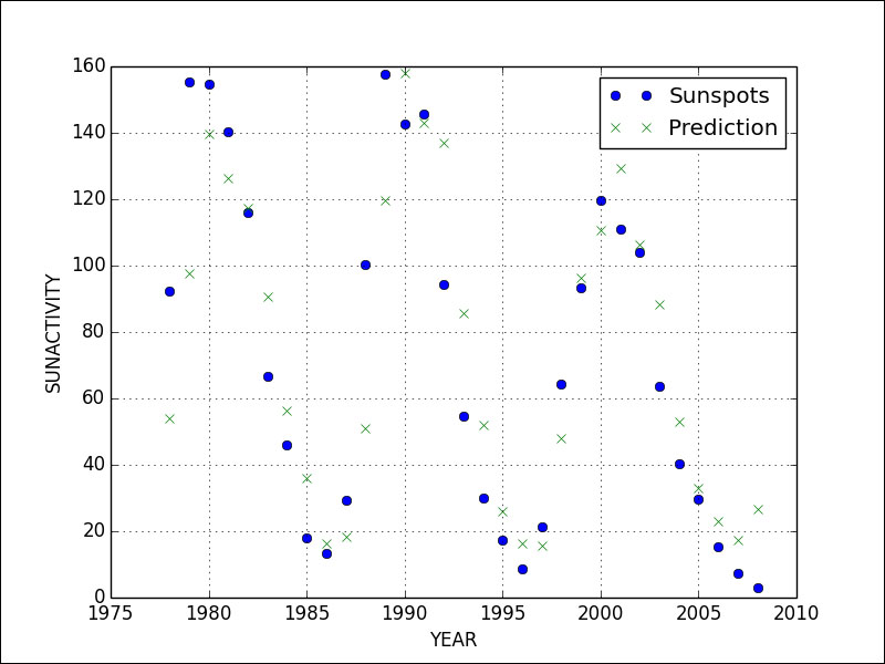
It seems that we have many predictions that are almost spot-on, but also a bunch of predictions that are pretty far off. Overall, we don't have a perfect fit; however, it's not a complete disaster. It's somewhere in the middle.
The following code is in the ar.py file in this book's code bundle:
from scipy.optimize import leastsq
import statsmodels.api as sm
import matplotlib.pyplot as plt
import numpy as np


def model(p, x1, x10):
   p1, p10 = p
   return p1 * x1 + p10 * x10

def error(p, data, x1, x10):
   return data - model(p, x1, x10)

def fit(data):
   p0 = [.5, 0.5]
   params = leastsq(error, p0, args=(data[10:], data[9:-1], data[:-10]))[0]
   return params

data_loader = sm.datasets.sunspots.load_pandas()
sunspots = data_loader.data["SUNACTIVITY"].values

cutoff = .9 * len(sunspots)
params = fit(sunspots[:cutoff])
print "Params", params

pred = params[0] * sunspots[cutoff-1:-1] + params[1] * sunspots[cutoff-10:-10]
actual = sunspots[cutoff:]
print "Root mean square error", np.sqrt(np.mean((actual - pred) ** 2))
print "Mean absolute error", np.mean(np.abs(actual - pred))
print "Mean absolute percentage error", 100 * np.mean(np.abs(actual - pred)/actual)
mid = (actual + pred)/2
print "Symmetric Mean absolute percentage error", 100 * np.mean(np.abs(actual - pred)/mid)
print "Coefficient of determination", 1 - ((actual - pred) ** 2).sum()/ ((actual - actual.mean()) ** 2).sum()
year_range = data_loader.data["YEAR"].values[cutoff:]
plt.plot(year_range, actual, 'o', label="Sunspots")
plt.plot(year_range, pred, 'x', label="Prediction")
plt.grid(True)
plt.xlabel("YEAR")
plt.ylabel("SUNACTIVITY")
plt.legend()
plt.show()