The binomial distribution models the number of successes in an integer number of independent runs of an experiment, where the chance of success in each experiment is a set number.

Envisage a 17th-century gambling house where you can wager on tossing pieces of eight. Nine coins are flipped in a popular game. If less than five coins are heads, then you lose one piece of eight; otherwise, you earn one. Let's simulate this, commencing with one thousand coins in our possession. We will use the binomial() function from the random module for this purpose:

import numpy as np
from matplotlib.pyplot import plot, show

cash = np.zeros(10000)
cash[0] = 1000
outcome = np.random.binomial(9, 0.5, size=len(cash))

for i in range(1, len(cash)):

   if outcome[i] < 5:
      cash[i] = cash[i - 1] - 1
   elif outcome[i] < 10:
      cash[i] = cash[i - 1] + 1
   else:
      raise AssertionError("Unexpected outcome " + outcome)

print outcome.min(), outcome.max()

plot(np.arange(len(cash)), cash)
show()

In order to understand the binomial() function, take a look at the following steps:

You can determine in the following plot that our cash balance executes a random walk (random movement not following a pattern):

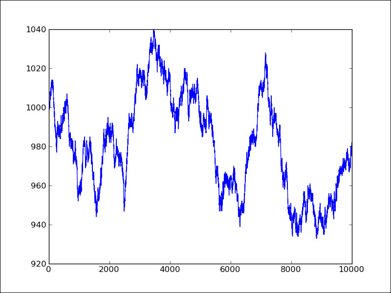
Of course, each time we execute the code, we will have a different random walk. If you want to always receive the same results, you will want to hand a seed value to the binomial() function from the NumPy random subpackage.

Continuous distributions are modeled by the probability density functions (pdf). The chance for a specified interval is found by integration of the probability density function. The NumPy random module has a number of functions that represent continuous distributions, such as beta, chisquare, exponential, f, gamma, gumbel, laplace, lognormal, logistic, multivariate_normal, noncentral_chisquare, noncentral_f, normal, and others.

We will visualize the normal distribution by applying the normal() function from the random NumPy subpackage. We will do this by drawing a bell curve and histogram of randomly generated values (refer to normaldist.py in this book's code bundle):

import numpy as np
import matplotlib.pyplot as plt

N=10000

normal_values = np.random.normal(size=N)
dummy, bins, dummy = plt.hist(normal_values, np.sqrt(N), normed=True, lw=1)
sigma = 1
mu = 0
plt.plot(bins, 1/(sigma * np.sqrt(2 * np.pi)) * np.exp( - (bins - mu)**2 / (2 * sigma**2) ),lw=2)
plt.show()

Random numbers can be produced from a normal distribution and their distribution might be displayed with a histogram. To plot a normal distribution, follow the ensuing steps:

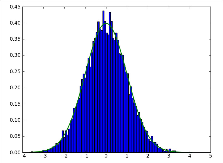
The normal distribution is widely used in science and statistics. According to the central limit theorem, a large, random sample with independent observations will converge towards the normal distribution. The properties of the normal distribution are well known and it is considered convenient to use. However, there are a number of requirements that need to be met such as a sufficiently large number of data points, and these data points must be independent. It is a good practice to check whether data conforms to the normal distribution or not. A great number of normality tests exist, some of which have been implemented in the scipy.stats package. We will apply these tests in this section. As sample data, we will use flu trends data from https://www.google.org/flutrends/data.txt. The original file has been reduced to include only two columns: a date and values for Argentina. A few lines are given as follows:

Date,Argentina
29/12/02,
05/01/03,
12/01/03,
19/01/03,
26/01/03,
02/02/03,136

The data can be found in the goog_flutrends.csv file of the code bundle. We will also sample data from the normal distribution as we did in the previous tutorial. The resulting array will have the same size as the flu trends array and will serve as the golden standard, which should pass the normality test with flying colors.

import numpy as np
from scipy.stats import shapiro
from scipy.stats import anderson
from scipy.stats import normaltest



flutrends = np.loadtxt("goog_flutrends.csv", delimiter=',', usecols=(1,), skiprows=1, converters = {1: lambda s: float(s or 0)}, unpack=True)
N = len(flutrends)
normal_values = np.random.normal(size=N)
zero_values = np.zeros(N)

print "Normal Values Shapiro", shapiro(normal_values)
print "Zeroes Shapiro", shapiro(zero_values)
print "Flu Shapiro", shapiro(flutrends)
print

print "Normal Values Anderson", anderson(normal_values)
print "Zeroes Anderson", anderson(zero_values)
print "Flu Anderson", anderson(flutrends)
print

print "Normal Values normaltest", normaltest(normal_values)
print "Zeroes normaltest", normaltest(zero_values)
print "Flu normaltest", normaltest(flutrends)

As a negative example, we will use an array of the same size as the two previously mentioned arrays filled with zeros. In real life, we could get this kind of values if we were dealing with a rare event (for instance, a pandemic outbreak).

In the data file, some cells are empty. Of course, these types of issues occur frequently, so we have to get used to cleaning our data. We are going to assume that the correct value should be 0. A converter can fill in those 0 values for us as follows:

flutrends = np.loadtxt("goog_flutrends.csv", delimiter=',', usecols=(1,), skiprows=1, converters = {1: lambda s: float(s or 0)}, unpack=True)

The Shapiro-Wilk test can check for normality. The corresponding SciPy function returns a tuple of which the first number is a test statistic and the second number is a p-value. It should be noted that the zeros-filled array caused a warning. In fact, all the three functions used in this example had trouble with this array and gave warnings. We get the following result:

Normal Values Shapiro (0.9967482686042786, 0.2774980068206787)
Zeroes Shapiro (1.0, 1.0)
Flu Shapiro (0.9351990818977356, 2.2945883254311397e-15)

The result for the zeros-filled array is a bit strange. Since we get a warning, it might be advisable to even ignore it altogether. The p-values we get are similar to the results of the third test later in this example. The analysis is basically the same.

The Anderson-Darling test can check for normality and also for other distributions such as Exponential, Logistic, and Gumbel. The related SciPy function related a test statistic and an array containing critical values for the 15, 10, 5, 2.5, and 1 percentage significance levels. If the statistic is larger than the critical value at a significance level, we can reject normality. We get the following values:

Normal Values Anderson (0.31201465602225653, array([ 0.572,  0.652,  0.782,  0.912,  1.085]), array([ 15. ,  10. ,   5. ,   2.5,   1. ]))
Zeroes Anderson (nan, array([ 0.572,  0.652,  0.782,  0.912,  1.085]), array([ 15. ,  10. ,   5. ,   2.5,   1. ]))
Flu Anderson (8.258614154768793, array([ 0.572,  0.652,  0.782,  0.912,  1.085]), array([ 15. ,  10. ,   5. ,   2.5,   1. ]))

For the zeros-filled array, we cannot say anything sensible because the statistic returned is not a number. We are not allowed to reject normality for our golden standard array, as we would have expected. However, the statistic returned for the flu trends data is larger than all the corresponding critical values. We can, therefore, confidently reject normality. Out of the three test functions, this one seems to be the easiest to use.

The D'Agostino and Pearson's test is also implemented in SciPy as the normaltest() function. This function returns a tuple with a statistic and p-value just like the shapiro() function. The p-value is a two-sided Chi-squared probability. Chi-squared is another well-known distribution. The test itself is based on z-scores of the skewness and kurtosis tests. Skewness measures how symmetric a distribution is. The normal distribution is symmetric and has zero skewness. Kurtosis tells us something about the shape of the distribution (high peak, fat tail). The normal distribution has a kurtosis of three (the excess kurtosis is zero). The following values are obtained by the test:

Normal Values normaltest (3.102791866779639, 0.21195189649335339)
Zeroes normaltest (1.0095473240349975, 0.60364218712103535)
Flu normaltest (99.643733363569538, 2.3048264115368721e-22)

Since we are dealing with a probability for the p-value, we want this probability to be as high as possible and close to one. For the zeros-filled array, this has strange consequences, but since we got warnings, the result for that particular array is not reliable. Further, we can accept normality if the p-value is at least 0.5. For the golden standard array, we get a lower value, which means that we probably need to have more observations. It is left as an exercise for you to confirm this.