This is the most controversial section in the book so far. Genetic algorithms are based on the biological theory of evolution (see http://en.wikipedia.org/wiki/Evolutionary_algorithm). This type of algorithm is useful for searching and optimization. For instance, we can use it to find the optimal parameters for a regression or classification problem.

Humans and other life forms on Earth carry genetic information in chromosomes. Chromosomes are frequently modeled as strings. A similar representation is used in genetic algorithms. The first step is to initialize the population with random individuals and related representation of genetic information. We can also initialize with already-known candidate solutions for the problem. After that, we go through many iterations called generations. During each generation, individuals are selected for mating based on a predefined fitness function. The fitness function evaluates how close an individual is to the desired solution.

Two genetic operators generate new genetic information:

Eventually, the new individuals replace the old population and we can start a new iteration. In this example, we will use the Python DEAP library. Install DEAP as follows:

$ sudo pip install deap
$ pip freeze|grep deap
deap==1.0.1

Start by defining a Fitness subclass that maximizes fitness:

creator.create("FitnessMax", base.Fitness, weights=(1.0,))

Then, define a template for each individual in the population:

creator.create("Individual", array.array, typecode='d', fitness=creator.FitnessMax)

DEAP has the concept of a toolbox, which is a registry of necessary functions. Create a toolbox and register the initialization functions, as follows:

toolbox = base.Toolbox()
toolbox.register("attr_float", random.random)
toolbox.register("individual", tools.initRepeat, creator.Individual, toolbox.attr_float, 200)
toolbox.register("populate", tools.initRepeat, list, toolbox.individual)

The first function generates floating-point numbers between 0 and 1. The second function creates an individual with a list of 200 floating point numbers. The third function creates a list of individuals. This list represents the population of possible solutions for a search or optimization problem.

In a society, we want "normal" individuals, but also people like Einstein. In Chapter 3, Statistics and Linear Algebra, we were introduced to the shapiro() function, which performs a normality test. For an individual to be normal, we require that the normality test p-value of his or her list to be as high as possible. The following code defines the fitness function:

def eval(individual):
    return shapiro(individual)[1],

Let's define the genetic operators:

toolbox.register("evaluate", eval)
toolbox.register("mate", tools.cxTwoPoint)
toolbox.register("mutate", tools.mutFlipBit, indpb=0.1)
toolbox.register("select", tools.selTournament, tournsize=4)

The following list will give you an explanation about the preceding genetic operators:

In the preceding code snippet, we specified that we are going to use two-point crossover and the probability of an attribute to be flipped. Generate 400 individuals as the initial population:

pop = toolbox.populate(n=400)

Now start the evolution process, as follows:

hof = tools.HallOfFame(1)
stats = tools.Statistics(key=lambda ind: ind.fitness.values)
stats.register("max", np.max)

algorithms.eaSimple(pop, toolbox, cxpb=0.5, mutpb=0.2, ngen=80, stats=stats, halloffame=hof)

The program reports statistics including the maximum fitness for each generation. We specified the crossover probability, mutation rate, and maximum generations after which to stop. The following is an extract of the displayed statistics report:

gen        nevals        max
0          400           0.000484774
1          245           0.000776807
2          248           0.00135569
…
79         250           0.99826
80         248           0.99826

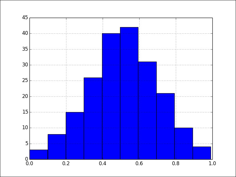
As you can see, we start out with distributions that are far from normal, but eventually we get an individual with the following histogram:

Refer to the gen_algo.py file in this book's code bundle:

import array
import random
import numpy as np
from deap import algorithms
from deap import base
from deap import creator
from deap import tools
from scipy.stats import shapiro
import matplotlib.pyplot as plt


creator.create("FitnessMax", base.Fitness, weights=(1.0,))
creator.create("Individual", array.array, typecode='d', fitness=creator.FitnessMax)

toolbox = base.Toolbox()
toolbox.register("attr_float", random.random)
toolbox.register("individual", tools.initRepeat, creator.Individual, toolbox.attr_float, 200)
toolbox.register("populate", tools.initRepeat, list, toolbox.individual)

def eval(individual):
    return shapiro(individual)[1],

toolbox.register("evaluate", eval)
toolbox.register("mate", tools.cxTwoPoint)
toolbox.register("mutate", tools.mutFlipBit, indpb=0.1)
toolbox.register("select", tools.selTournament, tournsize=4)

random.seed(42)

pop = toolbox.populate(n=400)
hof = tools.HallOfFame(1)
stats = tools.Statistics(key=lambda ind: ind.fitness.values)
stats.register("max", np.max)

algorithms.eaSimple(pop, toolbox, cxpb=0.5, mutpb=0.2, ngen=80, stats=stats, halloffame=hof)

print shapiro(hof[0])[1]
plt.hist(hof[0])
plt.grid(True)
plt.show()