IPython Parallel is the IPython API for parallel computing. We will set it up to use MPI for message passing. We may have to set environment variables as follows:

$ export LC_ALL=en_US.UTF-8
$ export LANG=en_US.UTF-8

Issue the following command at the command line:

$ ipython profile create --parallel --profile=mpi

The preceding command will create a file in our home directory, which can be found at .ipython/profile_mpi/iplogger_config.py.

Add the following line in this file:

c.IPClusterEngines.engine_launcher_class = 'MPIEngineSetLauncher'

Start a cluster that uses the MPI profile as follows:

$ ipcluster start -–profile=mpi --engines=MPI --debug

The preceding command specifies that we are using the mpi profile and MPI engine with debug-level logging. We can now interact with the cluster from an IPython Notebook. Start a notebook with plotting enabled and with NumPy, SciPy, and matplotlib automatically imported as follows:

$ ipython notebook --profile=mpi --log-level=DEBUG --pylab inline

The preceding command uses the mpi profile with debug log level. The notebook for this example is stored in the IPythonParallel.ipynb file in this book's code bundle. Import the IPython Parallel Client class and the statsmodels.api module as follows:

  In [1]:from IPython.parallel import Client
  import statsmodels.api as sm

Load the sunspots data and calculate the mean:

  In [2]: data_loader = sm.datasets.sunspots.load_pandas()
  vals = data_loader.data['SUNACTIVITY'].values
  glob_mean = vals.mean()
  glob_mean

The following will be output:

Out [2]: 49.752103559870541

Create a client as follows:

In [3]: c = Client(profile='mpi')

Create a view to the clients with the following line:

In [4]: view=c[:]

IPython has the concept of magics. These are special commands specific to IPython notebooks. Enable magics as follows:

In [5]: view.activate()

Load the mpi_ipython.py file in this book's code bundle:

from mpi4py import MPI
from numpy.random import random_integers
from numpy.random import randn
import numpy as np
import statsmodels.api as sm
import bottleneck as bn
import logging


def jackknife(a, parallel=True):
    data_loader = sm.datasets.sunspots.load_pandas()
    vals = data_loader.data['SUNACTIVITY'].values

    func, _ = bn.func.nanmean_selector(vals, axis=0)
    results = []

    for i in a:
        tmp = np.array(vals.tolist())
        tmp[i] = np.nan
        results.append(func(tmp))
    results = np.array(results)

    if parallel:
        comm = MPI.COMM_WORLD
        rcvBuf = np.zeros(0.0, 'd')
        comm.gather([results, MPI.DOUBLE], [rcvBuf, MPI.DOUBLE])

   return results

if __name__ == "__main__":
    skiplist = np.arange(39, dtype='int')
    print jackknife(skiplist, False)

The preceding program contains a function, which performs jackknife resampling. Jackknife resampling is a type of resampling where we omit one of the observations in the sample and then calculate the statistical estimator we are interested in. In this case, we are interested in the mean. We leave one observation out by setting it to NumPy NaN. Then, we call the Bottleneck nanmean() function on the new sample. The following is the load command:

In [6]: view.run('mpi_ipython.py')

Next, we split and spread an array with all the indices of the sunspots array:

In [7]: view.scatter('a',np.arange(len(vals),dtype='int'))

The a array can be displayed in the notebook as follows:

In [8]: view['a']

Here is the output of the preceding command:

Out[8]:[array([ 0,  1,  2,  3,  4,  5,  6,  7,  8,  9, 10, 11, 12, 13, 14, 15, 16,  17, 18, 19, 20, 21, 22, 23, 24, 25, 26, 27, 28, 29, 30, 31, 32, 33,  34, 35, 36, 37, 38]), … TRUNCATED …]

Call the jackknife() function on all the clients:

In [9]: %px means = jackknife(a)

Once all the worker processes are done, we can view the result:

In [10]: view['means']

The result is a list of as many processes as we started. Each process returns a NumPy array containing means calculated by jackknife resampling. This structure is not very useful, so transform it into a flat list:

In [11]: all_means = []

for v in view['means']:
    all_means.extend(v)

mean(all_means)

You will get the following output:

Out [11]: 49.752103559870577

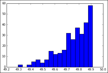
We can also compute the standard deviation, but that is easy so we will skip it. It's much more interesting to plot a histogram of the jackknifed means:

In [13]: hist(all_means, bins=sqrt(len(all_means)))

Refer to the following plot for the end result:

For troubleshooting, we can use the following line that displays error messages from the worker processes:

In [14]: [(k, c.metadata[k]['started'], c.metadata[k]['pyout'], c.metadata[k]['pyerr']) for k in c.metadata.keys()]