Many natural phenomena are regular and trustworthy like an accurate clock. Some phenomena exhibit patterns that seem regular. A group of scientists found three cycles in the sunspot activity with the
Hilbert-Huang transform (see http://en.wikipedia.org/wiki/Hilbert%E2%80%93Huang_transform). The cycles have a duration of 11, 22, and 100 years approximately. Normally, we would simulate a periodic signal using trigonometric functions such as a sine function. You probably remember a bit of trigonometry from high school. That's all we need for this example. Since we have three cycles, it seems reasonable to create a model, which is a linear combination of three sine functions. This just requires a tiny adjustment of the code for the autoregressive model. Refer to the periodic.py file in this book's code bundle for the following code:
from scipy.optimize import leastsq
import statsmodels.api as sm
import matplotlib.pyplot as plt
import numpy as np
def model(p, t):
C, p1, f1, phi1 , p2, f2, phi2, p3, f3, phi3 = p
return C + p1 * np.sin(f1 * t + phi1) + p2 * np.sin(f2 * t + phi2) +p3 * np.sin(f3 * t + phi3)
def error(p, y, t):
return y - model(p, t)
def fit(y, t):
p0 = [y.mean(), 0, 2 * np.pi/11, 0, 0, 2 * np.pi/22, 0, 0, 2 * np.pi/100, 0]
params = leastsq(error, p0, args=(y, t))[0]
return params
data_loader = sm.datasets.sunspots.load_pandas()
sunspots = data_loader.data["SUNACTIVITY"].values
years = data_loader.data["YEAR"].values
cutoff = .9 * len(sunspots)
params = fit(sunspots[:cutoff], years[:cutoff])
print "Params", params
pred = model(params, years[cutoff:])
actual = sunspots[cutoff:]
print "Root mean square error", np.sqrt(np.mean((actual - pred) ** 2))
print "Mean absolute error", np.mean(np.abs(actual - pred))
print "Mean absolute percentage error", 100 * np.mean(np.abs(actual - pred)/actual)
mid = (actual + pred)/2
print "Symmetric Mean absolute percentage error", 100 * np.mean(np.abs(actual - pred)/mid)
print "Coefficient of determination", 1 - ((actual - pred) ** 2).sum()/ ((actual - actual.mean()) ** 2).sum()
year_range = data_loader.data["YEAR"].values[cutoff:]
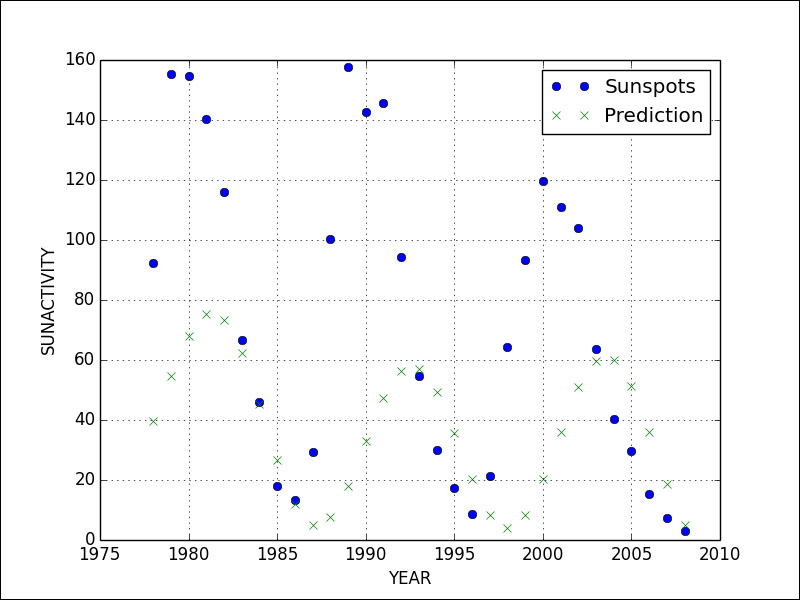
plt.plot(year_range, actual, 'o', label="Sunspots")
plt.plot(year_range, pred, 'x', label="Prediction")
plt.grid(True)
plt.xlabel("YEAR")
plt.ylabel("SUNACTIVITY")
plt.legend()
plt.show()Params [ 47.18800285 28.89947419 0.56827284 6.51168446 4.55214999 0.29372077 -14.30926648 -18.16524041 0.06574835 -4.37789602] Root mean square error 59.5619175499 Mean absolute error 44.5814573306 Mean absolute percentage error 65.1639657495 Symmetric Mean absolute percentage error 78.4477263927 Coefficient of determination -0.363525210982
The first line displays the coefficients of the model we attempted. We have a mean absolute error of 44, which means that we are off by that amount in either direction on average. We also want the coefficient of determination to be as close to one as possible to have a good fit. Instead, we get a negative value, which is undesirable. Refer to the following graph for the end result: