The mode is the integer that appears the maximum number of times in the dataset. It happens to be the value with the highest frequency in the dataset. In the x dataset in the median example, the mode is 2 because it occurs twice in the set.

Python provides different libraries for operating descriptive statistics in the dataset. Commonly used libraries are pandas, numpy, and scipy. These measures of central tendency can simply be calculated by the numpy and pandas functionalities.

To practice descriptive statistics, we would require a dataset that has multiple numerical records in it. Here is a dataset of automobiles that enlists different features and attributes of cars, such as symboling, normalized losses, aspiration, and many others, an analysis of which will provide some valuable insight and findings in relation to automobiles in this dataset.

Let's begin by importing the datasets and the Python libraries required:

import pandas as pd
import numpy as np

Now, let's load the automobile database:

df = pd.read_csv("data.csv")
df.head()

In the preceding code, we assume that you have the database stored in your current drive. Alternatively, you can change the path to the correct location. By now, you should be familiar with data loading techniques. The output of the code is given here:

Now, let's start by computing measures of central tendencies. Before establishing these for all the rows, let's see how we can get central tendencies for a single column. For example, we want to obtain the mean, median, and mode for the column that represents the height. In pandas, we can get an individual column easily by specifying the column name as dataframe["column_name"]. In our case, our DataFrame is stored in the df variable. Hence, we can get all the data items for height as df["height"]. Now, pandas provides easy built-in functions to measure central tendencies. Let's compute this as follows:

height =df["height"]
mean = height.mean()
median =height.median()
mode = height.mode()
print(mean , median, mode)

The output of the preceding code is as follows:

53.766666666666715 54.1 0 50.8
dtype: float64

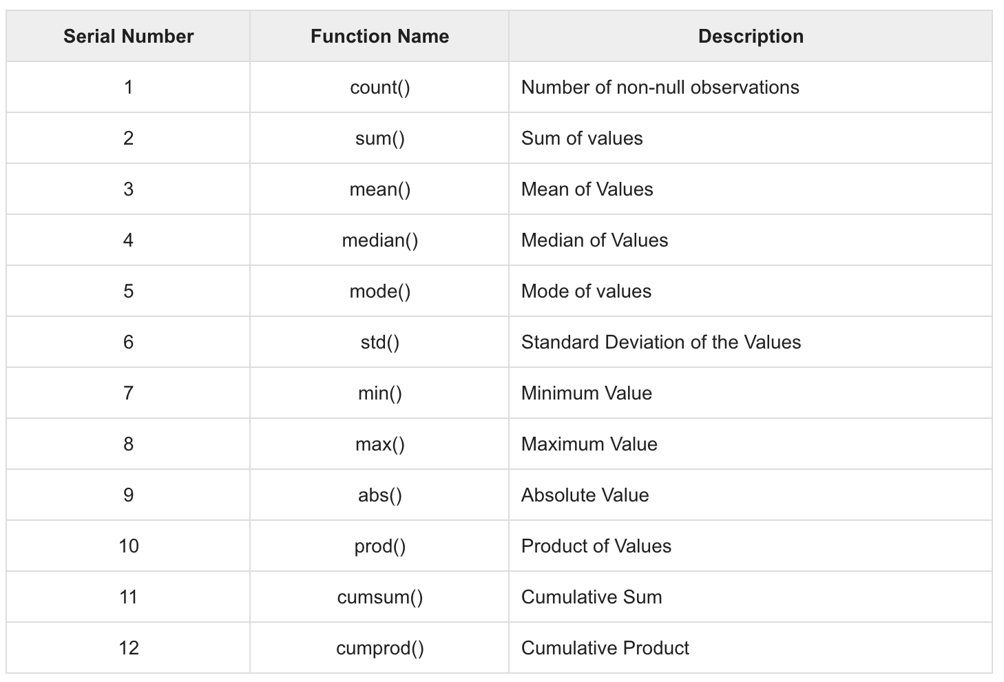
Now, the important thing here is to interpret the results. Just with these simple statistics, we can understand that the average height of the cars is around 53.766 and that there are a lot of cars whose mode value is 50.8. Similarly, we can get measures of the central tendencies for any columns whose data types are numeric. A list of similar functions that are helpful is shown in the following screenshot:

In addition to finding statistics for a single column, it is possible to find descriptive statistics for the entire dataset at once. Pandas provides a very useful function, df.describe, for doing so:

df.describe()

The output of the preceding code is shown in the following screenshot:

If you have used pandas before, I am pretty sure you have heard about or probably used this function several times. But have you really understood the output you obtained? In the preceding table, you can see that we have statistics for all the columns, excluding NaN values. The function takes both numeric and objects series under consideration during the calculation. In the rows, we get the count, mean, standard deviation, minimum value, percentiles, and maximum values of that column. We can easily understand our dataset in a better way. In fact, if you check the preceding table, you can answer the following questions:

• What is the total number of rows we have in our dataset?
• What is the average length, width, height, price, and compression ratio of the cars?
• What is the minimum height of the car? What is the maximum height of the car?
• What is the maximum standard deviation of the curb weight of the cars?. 

We can now, in fact, answer a lot of questions, just based on one table. Pretty good, right? Now, whenever you start any data science work, it is always considered good practice to perform a number of sanity checks. By sanity checks, I mean understanding your data before actually fitting machine learning models. Getting a description of the dataset is one such sanity check.  

In the case of categorical variables that have discrete values, we can summarize the categorical data by using the value_counts() function. Well, an example is better than a precept. In our dataset, we have a categorical data column, make. Let's first count the total number of entries according to such categories, and then take the first 30 largest values and draw a bar chart:

df.make.value_counts().nlargest(30).plot(kind='bar', figsize=(14,8))
plt.title("Number of cars by make")
plt.ylabel('Number of cars')
plt.xlabel('Make of the cars')

By now, the preceding code should be pretty familiar. We are using the value_counts() function from the pandas library. Once we have the list, we are getting the first 30 largest values by using the nlargest() function. Finally, we exploit the plot function provided by the pandas library. The output of the preceding code snippet is shown here:

The table, as shown, is helpful. To add a degree of comprehension, we can use visualization techniques as shown in the preceding diagram. It is pretty clear from the diagram that Toyota's brand is the most popular brand. Similarly, we can easily visualize successive brands on the list.