Let's next find out which of the columns from the red wine database are highly correlated. If you recall, we discussed different types of correlation in Chapter 7, Correlation. Just so you grasp the intention behind the correlation, I highly recommend going through Chapter 7, Correlation, just to revamp your memory. Having said that, let's continue with finding highly correlated columns: 

1. We can continue using the seaborn.pairplot() method, as shown here:

sns.pairplot(df_red)

And you should get a highly comprehensive graph, as shown in the screenshot:

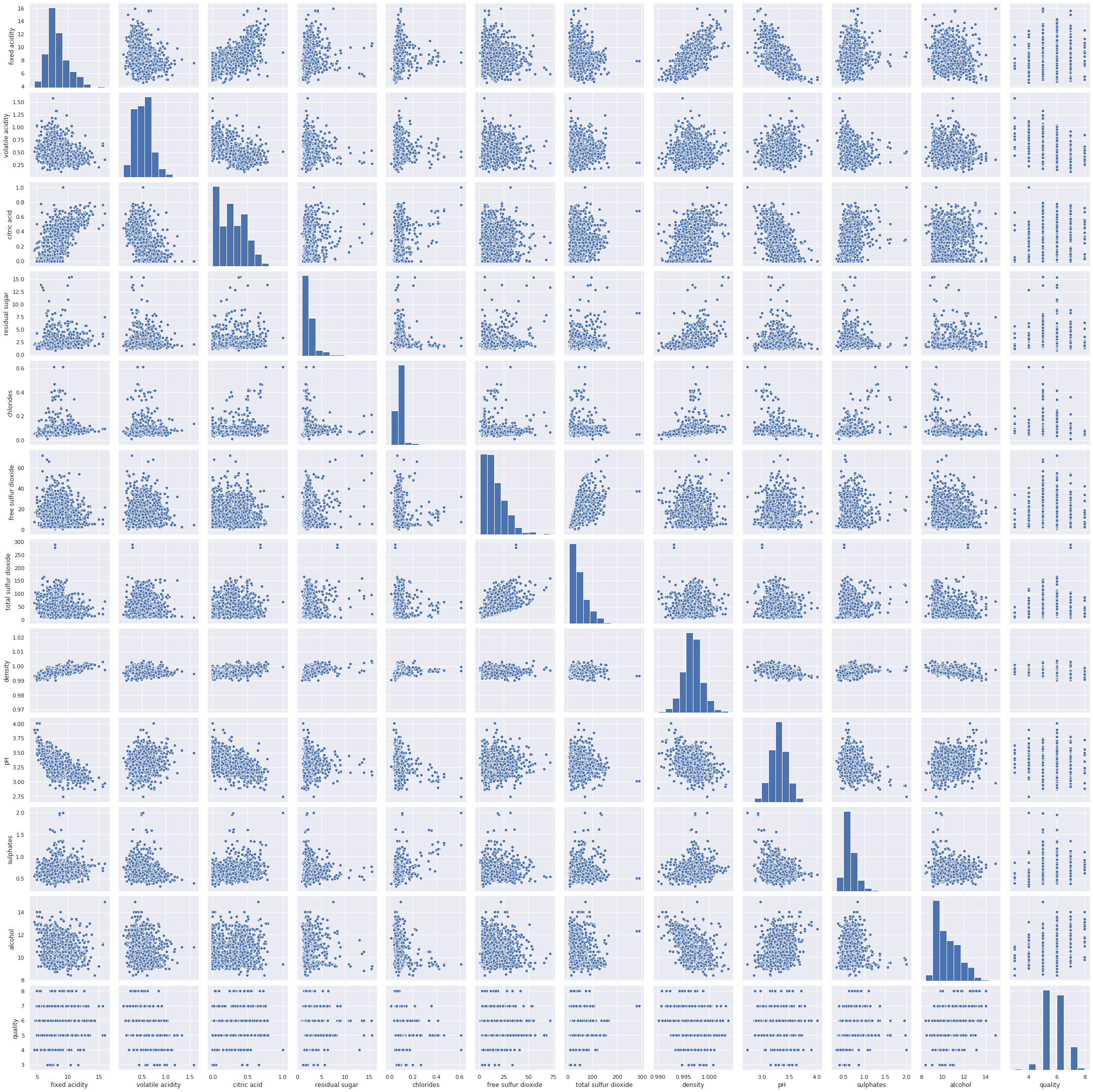
The preceding screenshot shows scattered plots for every possible combination pair of columns. The graph illustrates some positive correlation between fixed acidity and density. There is a negative correlation of acidity with pH. Similarly, there is a negative correlation between alcohol percentage and density. Moreover, you can exactly see which columns have a positive or negative correlation with other columns. However, since there are no numbers of the pairplot graph, it might be a bit biased to interpret the results. For example, examine the correlation between the columns for the fixed acidity and the volatile acidity. The graph might be somehow symmetric. However, you might argue there are some sparse points on the right side of the graph so there's lightly negative correlation. Here, my point is, without any specific quantifiable number, it is hard to tell. This is the reason why we can use the sns.heatmap() method to quantify the correlation. 

2. We can generate the heatmap graph, as shown here:

sns.heatmap(df_red.corr(), annot=True, fmt='.2f', linewidths=2)

And the output it generates is as follows:

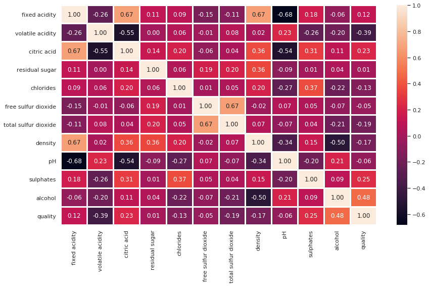
Figure 12.5 depicts the correlation between different columns. Since we are focusing on the quality column, the quality column has a positive correlation with alcohol, sulfates, residual sugar, citric acid, and fixed acidity. Since there are numbers, it is easy to see which columns are positively correlated and which columns are negatively correlated. 

Look at Figure 12.5 and see whether you can draw the following conclusions:

• Alcohol is positively correlated with the quality of the red wine. 
• Alcohol has a weak positive correlation with the pH value. 
• Citric acid and density have a strong positive correlation with fixed acidity. 
• pH has a negative correlation with density, fixed acidity, citric acid, and sulfates. 

There are several conclusions we can draw from the heatmap in Figure 12.5. Moreover, it is essential we realize the significance of the correlation and how it can benefit us in deciding feature sets during data science model development. 

We can further dive into individual columns and check their distribution. Say, for example, we want to see how alcohol concentration is distributed with respect to the quality of the red wine. First, let's plot the distribution plot, as shown here:

sns.distplot(df_red['alcohol'])

The output of the preceding code is as follows:

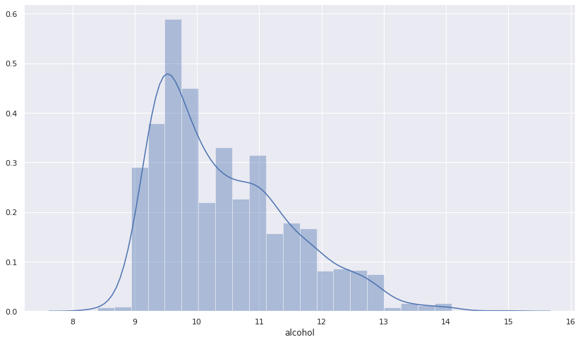
From Figure 12.6, we can see that alcohol distribution is positively skewed with the quality of the red wine. We can verify this using the skew method from scipy.stats. Check the snippet given here:

from scipy.stats import skew
skew(df_red['alcohol'])

And the output of the preceding code is as follows:

0.8600210646566755

The output verifies that alcohol is positively skewed. That gives deeper insight into the alcohol column.  

Note that we can verify each column and try to see their skewness, distribution, and correlation with respect to the other column. This is generally essential as we are going through the process of feature engineering.