In this section, we are going to develop different types of classical ML models and evaluate their performances. We have already discussed in detail the development of models and their evaluation in Chapter 9, Hypothesis Testing and Regression and Chapter 10, Model Development and Evaluation. Here, we will dive directly into implementation. 

We are going to use different types of following algorithms and evaluate their performances:

• Logistic regression
• Support vector machine
• K-nearest neighbor classifier
• Random forest classifier
• Decision tree classifier
• Gradient boosting classifier
• Gaussian Naive Bayes classifier

While going over each classifier in depth is out of the scope of this chapter and book, our aim here is to present how we can continue developing ML algorithms after performing EDA operations on certain databases: 

1. Let's first import the required libraries:

from sklearn.linear_model import LogisticRegression
from sklearn.svm import LinearSVC,SVC
from sklearn.neighbors import KNeighborsClassifier
from sklearn.ensemble import RandomForestClassifier,GradientBoostingClassifier,AdaBoostClassifier
from sklearn.tree import DecisionTreeClassifier
from sklearn.naive_bayes import GaussianNB
from sklearn.model_selection import train_test_split,cross_validate
from sklearn.preprocessing import MinMaxScaler,StandardScaler,LabelEncoder
from sklearn.metrics import accuracy_score,precision_score,recall_score,f1_score 

Note that we are going to use the combined dataframe. Next, we are going to encode the categorical values for the quality_label column. We will encode the values so that all of the low values will be changed to 0, the medium values will be changed to 1, and the high values will be changed to 2.

2. Let's perform the encoding:

label_quality = LabelEncoder()

df_wines['quality_label'] = label_quality.fit_transform(df_wines['quality_label'])

That was not difficult, right? We just utilized the LabelEncoder utility function provided by the sklearn preprocessing functionality. 

3. Now, let's split our dataset into a training set and test set. We will use 70% of the dataset as the training set and the remaining 30% as the test set: 

x_train,x_test,y_train,y_test=train_test_split(df_wines.drop(['quality','wine_category'],axis=1),df_wines['quality_label'],test_size=0.30,random_state=42)

We used the train_test_split() method provided by the sklearn library. Note the following things in the preceding category:

• In the preceding code, we no longer need the quality and wine_category columns, so we drop them. 
• Next, we take 30% of the data as the test set. We can do that by simply passing the test_size = 0.30 argument.

4. Next, we create the model. Note that we could build the model individually for each of the algorithms we listed above. Instead, here we are going to list them and loop over each of them and compute the accuracy. Check the code snippet given as follows:

models=[LogisticRegression(),
        LinearSVC(),
        SVC(kernel='rbf'),
        KNeighborsClassifier(),
        RandomForestClassifier(),
        DecisionTreeClassifier(),
        GradientBoostingClassifier(),
        GaussianNB()]

model_names=['LogisticRegression','LinearSVM','rbfSVM', 'KNearestNeighbors', 'RandomForestClassifier', 'DecisionTree', 'GradientBoostingClassifier', 'GaussianNB']

5. Next, we will loop over each model, create a model, and then evaluate the accuracy. Check the code snippet given as follows:

acc=[]
eval_acc={}

for model in range(len(models)):
    classification_model=models[model]
    classification_model.fit(x_train,y_train)
    pred=classification_model.predict(x_test)
    acc.append(accuracy_score(pred,y_test))
     
eval_acc={'Modelling Algorithm':model_names,'Accuracy':acc}
eval_acc

The output of the preceding code is given here:

{'Accuracy': [0.9687179487179487,
  0.9733333333333334,
  0.6051282051282051,
  0.6912820512820513,
  1.0,
  1.0,
  1.0,
  1.0],
 'Modelling Algorithm': ['LogisticRegression',
  'LinearSVM',
  'rbfSVM',
  'KNearestNeighbors',
  'RandomForestClassifier',
  'DecisionTree',
  'GradientBoostingClassifier',
  'GaussianNB']}

6. Let's create a dataframe of the accuracy and show it in a bar chart:

acc_table=pd.DataFrame(eval_acc)
acc_table = acc_table.sort_values(by='Accuracy', ascending=[False])
acc_table

The output of the preceding code is given as follows:

Note that converting quality into a categorical dataset gave us higher accuracy. Most of the algorithms gave 100% accuracy as shown in the previous screenshot.

7. Let's create a bar plot:

sns.barplot(y='Modelling Algorithm',x='Accuracy',data=acc_table)

The output of the preceding code is given as follows:

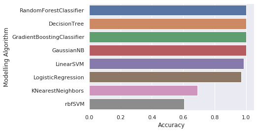
Note that, as shown in the screenshot, the random forest, the decision tree, the gradient boosting classifier, and the Gaussian Naive Bayes classifier all gave 100% accuracy.

Great! Congratulations, you have successfully completed the main project. Please note that all of the code, snippets, and methods illustrated in this book have been given to provide minimal ways in which a particular problem can be solved. There is always a way in which you can perform deeper analysis. We motivate you to go through the Further reading sections on each chapter to get advanced knowledge about the particular domain.