As its name suggests, this is the analysis of more than one (that is, exactly two) type of variable. Bivariate analysis is used to find out whether there is a relationship between two different variables. When we create a scatter plot by plotting one variable against another on a Cartesian plane (think of the x and y axes), it gives us a picture of what the data is trying to tell us. If the data points seem to fit the line or curve, then there is a relationship or correlation between the two variables. Generally, bivariate analysis helps us to predict a value for one variable (that is, a dependent variable) if we are aware of the value of the independent variable. 

Here's a diagram showing a scatter plot of advertising dollars and sales rates over a period of time:

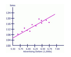
This diagram is the scatter plot for bivariate analysis, where Sales and Advertising Dollars are two variables. While plotting a scatter plot, we can see that the sales values are dependent on the advertising dollars; that is, as the advertising dollars increase, the sales values also increase. This understanding of the relationship between two variables will guide us in our future predictions:

1. It's now time to perform bivariate analysis on our automobiles dataset. Let's look at whether horsepower is a dependent factor for the pricing of cars or not:

# plot the relationship between “horsepower” and ”price”
plt.scatter(df["price"], df["horsepower"])
plt.title("Scatter Plot for horsepower vs price")
plt.xlabel("horsepower")
plt.ylabel("price")

This code will generate a scatter plot with a price range on the y axis and horsepower values on the x axis, as follows:

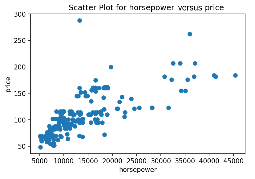
As you can see in the preceding diagram, the horsepower of cars is a dependent factor for the price. As the horsepower of a car increases, the price of the car also increases.

A box plot is also a nice way in which to view some statistical measures along with the relationship between two values.

2. Now, let's draw a box plot between the engine location of cars and their price:

#boxplot
sns.boxplot(x="engine-location",y="price",data=df)
plt.show()

This code will generate a box plot with the price range on the y axis and the types of engine locations on the x axis:

This diagram shows that the price of cars having a front engine-location is much lower than that of cars having a rear engine-location. Additionally, there are some outliers that have a front engine location but the price is much higher.

3. Next, plot another box plot with the price range and the driver wheel type:

#boxplot to visualize the distribution of "price" with types of "drive-wheels"
sns.boxplot(x="drive-wheels", y="price",data=df)

The output of this code is given as follows:

This diagram shows the range of prices of cars with different wheel types. Here, the box plot shows the average and median price in respective wheel types and some outliers too.

This was a brief introduction, along with a few practice examples of bivariate analysis. Now, let's learn about a more efficient type of practice for data analysis, multivariate analysis.