Remember the variables we worked with in Chapter 5, Descriptive Statistics, for measures of descriptive statistics? There we had a set of integers ranging from 2 to 12. We calculated the mean, median, and mode of that set and analyzed the distribution patterns of integers. Then, we calculated the mean, mode, median, and standard deviation of the values available in the height column of each type of automobile dataset. Such an analysis on a single type of dataset is called univariate analysis. 

Univariate analysis is the simplest form of analyzing data. It means that our data has only one type of variable and that we perform analysis over it. The main purpose of univariate analysis is to take data, summarize that data, and find patterns among the values. It doesn't deal with causes or relationships between the values. Several techniques that describe the patterns found in univariate data include central tendency (that is the mean, mode, and median) and dispersion (that is, the range, variance, maximum and minimum quartiles (including the interquartile range), and standard deviation).

Why don't you try doing an analysis over the same set of data again? This time, remember that this is univariate analysis:

1. Start by importing the required libraries and loading the dataset:

#import libraries
import matplotlib.pyplot as plt
import seaborn as sns
import pandas as pd

2. Now, load the data:

# loading dataset as Pandas dataframe
df = pd.read_csv("data.csv")
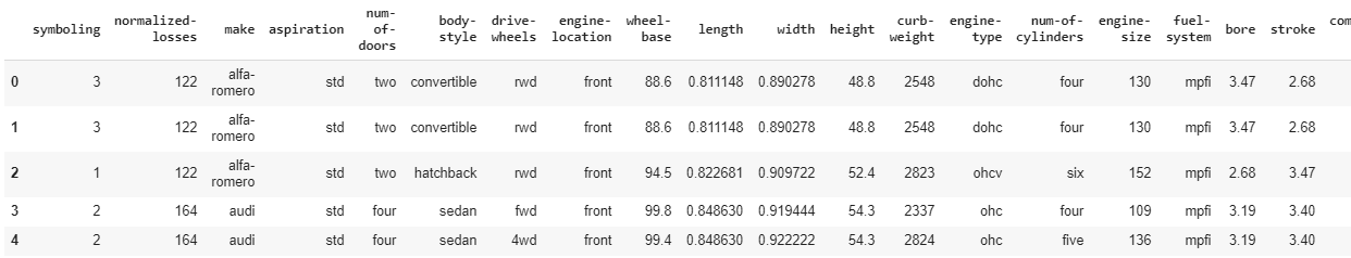
df.head()

The output of this code is given as follows:

3. First, check the data types of each column. By now, you must be familiar with the following:

df.dtypes

The output is as follows:

symboling int64
normalized-losses int64
make object
aspiration object
num-of-doors object
body-style object
drive-wheels object
engine-location object
wheel-base float64
length float64
width float64
height float64
curb-weight int64
engine-type object
num-of-cylinders object
engine-size int64
fuel-system object
bore float64
stroke float64
compression-ratio float64
horsepower float64
peak-rpm float64
city-mpg int64
highway-mpg int64
price float64
city-L/100km float64
horsepower-binned object
diesel int64
gas int64
dtype: object

4. Now compute the measure of central tendency of the height column. Recall that we discussed several descriptive statistics in Chapter 5, Descriptive Statistics:

#calculate mean, median and mode of dat set height
mean = df["height"].mean()
median =df["height"].median()
mode = df["height"].mode()
print(mean , median, mode)

The output of those descriptive functions is as follows:

53.766666666666715 54.1 0 50.8
dtype: float64

5. Now, let's visualize this analysis in the graph:

#distribution plot
sns.FacetGrid(df,size=5).map(sns.distplot,"height").add_legend()

The code will generate a distribution plot of values in the height column:

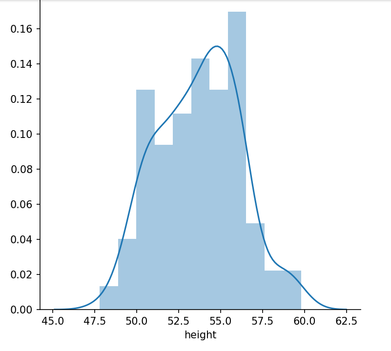
From the graph, we can observe that the maximum height of maximum cars ranges from 53 to 57. Now, let's do the same with the price column:

#distribution plot
sns.FacetGrid(df,size=5).map(sns.distplot,"price").add_legend()

The output of this code is given as follows:

Looking at this diagram, we can say that the price ranges from 5,000 to 45,000, but the maximum car price ranges between 5,000 and 10,000.

A box plot is also an effective method for the visual representation of statistical measures such as the median and quartiles in univariate analysis:

#boxplot for price of cars
sns.boxplot(x="price",data=df)
plt.show()

The box plot generated from the preceding code is given as follows:

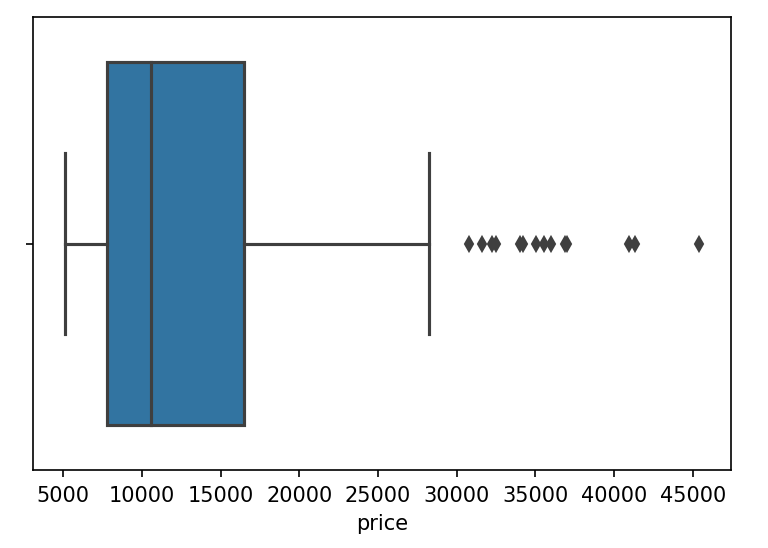
The right border of the box is Q3, that is, the third quartile, and the left border of the box is Q1, that is, the first quartile. Lines extend from both sides of the box boundaries toward the minimum and maximum. Based on the convention that our plotting tool uses, though, they may only extend to a certain statistic; any values beyond these statistics are marked as outliers (using points).

This analysis was for a dataset with a single type of variable only. Now, let's take a look at the next form of analysis for a dataset with two types of variables, known as bivariate analysis.