The first concept that comes to mind of any data science professional when solving any regression problem is to construct a linear regression model. Linear regression is one of the oldest algorithms, but it's still very efficient. We will build a linear regression model in Python using a sample dataset. This dataset is available in scikit-learn as a sample dataset called the Boston housing prices dataset. We will use the sklearn library to load the dataset and build the actual model. Let's start by loading and understanding the data:

1. Let's begin by importing all the necessary libraries and creating our dataframe:

# Importing the necessary libraries
import pandas as pd
import numpy as np
import matplotlib.pyplot as plt
import seaborn as sns 
from sklearn.datasets import load_boston

sns.set(style="ticks", color_codes=True)
plt.rcParams['figure.figsize'] = (8,5)
plt.rcParams['figure.dpi'] = 150

# loading the data
df = pd.read_csv("https://raw.githubusercontent.com/PacktPublishing/hands-on-exploratory-data-analysis-with-python/master/Chapter%209/Boston.csv")

2. Now, we have the dataset loaded into the boston variable. We can look at the keys of the dataframe as follows:

print(df.keys())

This returns all keys and values as the Python dictionary. The output of the preceding code is as follows:

Index(['CRIM', ' ZN ', 'INDUS ', 'CHAS', 'NOX', 'RM', 'AGE', 'DIS', 'RAD', 'TAX', 'PTRATIO', 'LSTAT', 'MEDV'], dtype='object')

3. Now that our data is loaded, let's get our DataFrame ready quickly and work ahead:

df.head()
# print the columns present in the dataset
print(df.columns)
# print the top 5 rows in the dataset
print(df.head()) 

The output of the preceding code is as follows:

The column MEDV is the target variable and, it will be used as the target variable while building the model. The target variable (y) is separate from the feature variable (x).

4. In the new overall dataframe, let's check if we have any missing values:

df.isna().sum()

Take a look at the following output:

CRIM 0
ZN 0
INDUS 0
CHAS 0
NOX 0
RM 0
AGE 0
DIS 0
RAD 0
TAX 0
PTRATIO 0
LSTAT 0
MEDV 0
dtype: int64

Particularly in the case of regression, it is important to make sure that our data does not have any missing values because regression won't work if the data has missing values.

Correlation analysis is a crucial part of building any model. We have to understand the distribution of the data and how the independent variables correlate with the dependent variable.

5. Let's plot a heatmap describing the correlation between the columns in the dataset:

#plotting heatmap for overall data set
sns.heatmap(df.corr(), square=True, cmap='RdYlGn')

The output plot looks like this:

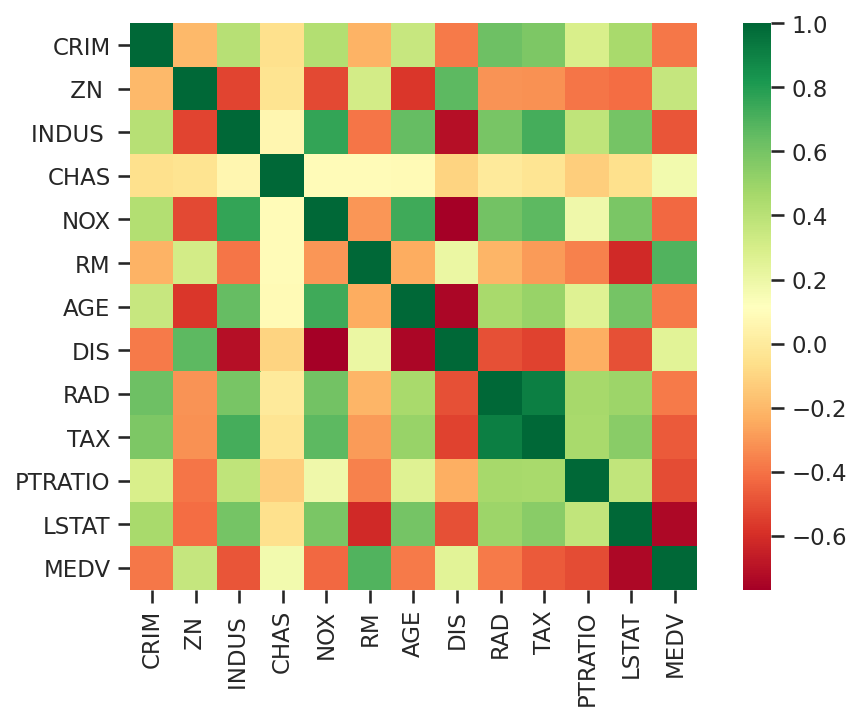
Since we want to build a linear regression model, let's look for a few independent variables that have a significant correlation with MEDV. From the preceding heatmap, RM (the average number of rooms per dwelling) has a positive correlation with MEDV (the median value of owner-occupied homes in $1,000s), so we will take RM as a feature (X) and MEDV as a predictor (y) for our linear regression model. 

6. We can use the lmplot method from seaborn to see the relationship between RM and MEDV. Check out the following snippet:

sns.lmplot(x = 'RM', y = 'MEDV', data = df)

The output of the preceding code is as follows:

The preceding screenshot shows a strong correlation between these two variables. However, there are some outliers that we can easily spot from the graph. Next, let's create grounds for model development. 

Scikit-learn needs to create features and target variables in arrays, so be careful when assigning columns to X and y:

# Preparing the data
X = df[['RM']]
y = df[['MEDV']]

And now we need to split our data into train and test sets. Sklearn provides methods through which we can split our original dataset into train and test datasets. As we already know, the reason behind the regression model development is to get a formula for predicting output in the future. But how can we be sure about the accuracy of the model's prediction? A logical technique for measuring the model's accuracy is to divide the number of correct predictions, by the total number of observations for the test.

For this task, we must have a new dataset with already known output predictions. The most commonly used technique for this during model development is called the train/test split of the dataset. Here, you divide the dataset into a training dataset and a testing dataset. We train, or fit, the model to the training dataset and then compute the accuracy by making predictions on the test (labeled or predicted) dataset.

7. This is done using the train_test_split() function available in sklearn.model_selection:

# Splitting the dataset into train and test sets
from sklearn.model_selection import train_test_split
X_train, X_test, y_train, y_test = train_test_split(X, y, test_size = 0.3, random_state = 10)

X is our independent variable here, and Y is our target (output) variable. In train_test_split, test_size indicates the size of the test dataset. test_size is the proportion of our data that is used for the test dataset. Here, we passed a value of 0.3 for test_size, which means that our data is now divided into 70% training data and 30% test data. Lastly, random_state sets the seed for the random number generator, which splits the data. The train_test_split() function will return four arrays: the training data, the testing data, the training outputs, and the testing outputs.

8. Now the final step is training the linear regression model. From the extremely powerful sklearn library, we import the LinearRegression() function to fit our training dataset to the model. When we run LinearRegression().fit(), the function automatically calculates the OLS, which we discussed earlier, and generates an appropriate line function:

#Training a Linear Regression Model
from sklearn.linear_model import LinearRegression
regressor = LinearRegression()

# Fitting the training data to our model
regressor.fit(X_train, y_train)

Now, we have a model called regressor that is fully trained on the training dataset. The next step is to evaluate how well the model predicts the target variable correctly.