Visual reports are new in Microsoft Office Project 2007 and are easy-to-build report templates that use Microsoft Office Excel 2003 or later (as well as Microsoft Office Visio Professional 2007) to transform Microsoft Project task, resource, and assignment information into charts and graphs that communicate your project information more effectively. For example, in earlier versions of Microsoft Project, displaying an Excel graph of earned value required special toolbars and numerous steps to produce the earned value status you wanted. In Microsoft Project 2007, you simply choose the Earned Value Over Time report, and the graph appears in Excel.
When you first start generating an Excel visual report, Microsoft Project gathers the information requested for the selected template and stores it in a database. Then, the visual report template calls on an Excel template to generate the report in an Excel PivotChart. Unlike Microsoft Project’s text-based reports, once data is set up for a visual report, you can configure the report to examine different fields over different time periods without generating a brand new report each time. For example, you could begin by analyzing cost overruns for each fiscal quarter and then drill down to view overruns by each week of the project. In addition, you can add, remove, or rearrange the fields you want to analyze.
You can modify existing visual reports or create your own report templates to do exactly what you want. You can use them on your own projects as well as publish them for other team members or project managers to use.
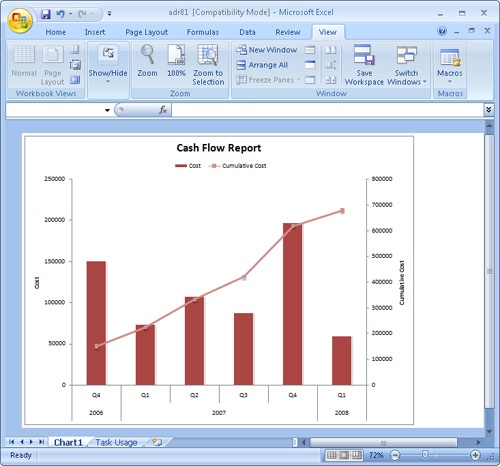
Unlike the text reports that are available in Microsoft Project 2007 and in earlier versions, visual reports transfer data to Excel and use Excel’s PivotTable feature to categorize and collate results. For example, suppose the executives on your project selection team ask to see cash flow by quarter for potential projects. Rather than use the text report of cash flow, which displays values for cash spent by time period, the Visual Cash Flow report generates an Excel chart that shows cash flows by quarter more clearly, as illustrated in Figure 17-29.
To generate a built-in visual report, do the following:
In Microsoft Project, click Reports, Visual Reports.
To view only those visual report templates that use Excel, clear the Microsoft Office Visio check box and be sure to select the Microsoft Office Excel check box.
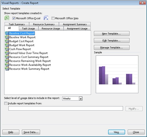
To view all the visual report templates that come with Microsoft Project, regardless of the category to which they belong, click the All tab (see Figure 17-30).
Figure 17-30. Specify whether you want to see report templates based on Excel or Visio and then select the report you want to generate.
Unless you create numerous custom visual report templates, it’s easy to find the reports you want on the All tab. However, if the list of reports grows unwieldy, select a category tab to see only the reports in that category. For example, the Task Usage category includes the Cash Flow Report template, whereas the Assignment Usage category includes templates for reporting baseline and budgeted costs and work as well as earned value over time.
To specify the level of detail that Microsoft Project transfers to Excel, click a time period (Days, Weeks, Months, Quarters, or Years) in the Select Level Of Usage Data To Include In The Report box.
For projects with shorter durations, choose Days or Weeks. If a project spans a year or more, consider using Months, Quarters, or even Years.
To generate the report, click View.
Excel launches and generates a PivotChart using the data transferred from Microsoft Project. The first worksheet in the Excel file, which contains the PivotChart, is called Chart1. The second worksheet is labeled with the name of the report category and contains the data for the report.
The built-in visual report templates cover many of the project status and performance topics that project managers need, such as baseline cost and work, cash flow, earned value, and resource availability. If none of the built-in reports do exactly what you want, you can edit a template to fit your requirements or create a new custom template.
Because visual reports use Excel PivotCharts or Visio Pivot Diagrams to do the heavy report lifting, visual report templates are either Excel or Visio templates. Whether you edit a built-in template or create your own, you specify the fields you want to work with and the type of data on which you want to report.
To edit a built-in visual report template, do the following:
Click Reports, Visual Reports.
Select the built-in visual report template you want to edit and then click Edit Template.
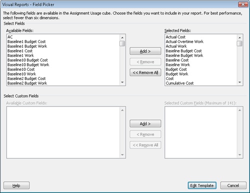
The Visual Reports Field Picker dialog box appears (see Figure 17-31).
To add fields to the OLAP cube for the visual report, in the Available Fields list, select the fields you want and then click Add.
The fields appear in the Selected Fields list. Remove fields from the Selected Fields list by selecting the ones you want to remove and then clicking Remove. You can select multiple fields to add or remove by holding the Ctrl key and clicking the fields.
Click the Edit Template button.
Microsoft Project builds the OLAP cube based on the fields you selected. Excel launches using the built-in Excel template.
Make the changes you want to the settings in Excel and then save the Excel template.
To create an Excel visual report template from scratch, do the following:
Click Reports, Visual Reports.
Click New Template.
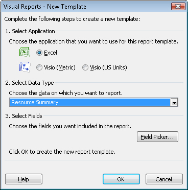
The Visual Reports New Template dialog box appears with the three basic selections you must make to build a template (see Figure 17-32).
If necessary, select the Excel option.
Under Select Data Type, choose the type of data you want to use as the basis for your report.
Visual reports are based on six different sets of information: Task Summary, Task Usage, Resource Summary, Resource Usage, Assignment Summary, and Assignment Usage. These data types determine the fields that Microsoft Project adds to the OLAP cube, but you can add or remove fields as well.
To modify the fields for the template, click Field Picker and add or remove fields in the Available Fields list.
To add fields to the new visual report’s OLAP cube, select the fields you want in the Available Fields list and then click Add.
To remove fields from the Selected Fields list, select the fields and then click Remove.
Click OK in the Visual Reports – Field Picker dialog box and then click OK in the Visual Reports – New Template dialog box.
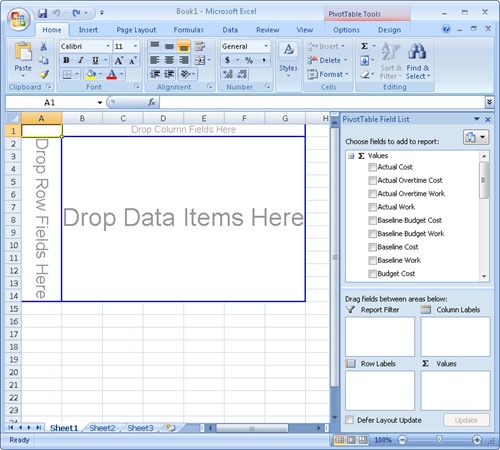
Excel launches and opens a blank PivotChart (see Figure 17-33).
To build the PivotTable, drag the field you want to use for rows in the table to the area labeled Drop Row Fields here. For example, to produce a resource report, drag the Resources field. Drag the field that you want to use for columns to the area labeled Drop Column Fields here, such as a time period for an earned value report.
Drag the Microsoft Project fields on which you want to report to the area labeled Drop Data Items Here.
When finished configuring the PivotTable, click the Microsoft Office Button and then click Save. In the Save As dialog box, make sure that the template is being saved to the folder where all the other templates are located. By default, this is in the UsersusernameAppDataRoamingMicrosoftTemplates1033 folder.
Saving the template in this folder ensures that the template will appear in the Visual Reports – Create Reports dialog box.
If you’d rather save your custom template in another location, you can still make it appear in the Visual Reports dialog box. In that dialog box, select the Include Reports Template From check box and click Modify to specify the path that contains your custom templates.
When Excel is open and displays one of your visual reports, you can use Excel PivotTable tools to configure what you see in the report. For example, you can change the time periods you see, add or remove fields in the chart, or display additional calculations.
Use one or more of the following techniques to change a visual report:
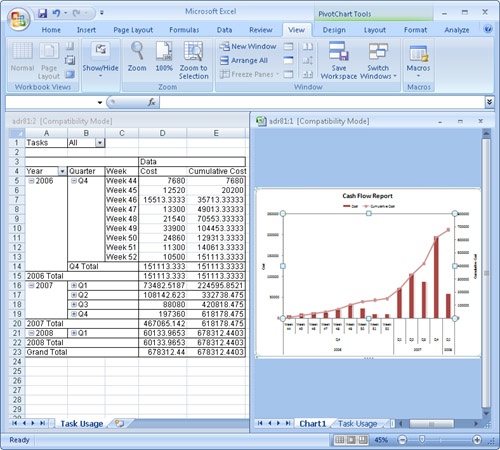
To control the totals that appear in the chart, click the tab for the data worksheet, such as Task Usage for the Cash Flow Report, and then expand or collapse the groupings in the table.
When data in the worksheet is collapsed as it is by default, you see plus signs to the left of collapsed groupings. For example, for a time-based report, Q1, Q2, Q3, and Q4 for each year are collapsed, but the years are expanded (indicated by a minus sign to the left). To show more detail for some or all of the report, click the plus sign next to the group you want to expand (see Figure 17-34).
To add fields within the chart, in the PivotTable Field list, select the check box for the field you want to add.
To remove a field, clear its check box.
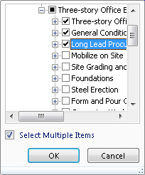
To filter the tasks, resources, or assignments included in the report, in the worksheet, click the down arrow in the first row. Expand the dropdown list to the level you want to see and then select the items you want to include (see Figure 17-35).
To change the calculation that appears in the chart, in the ∑ Values section, right click a field and then click Value Field Settings. In the Value Fields Settings dialog box, in the Summarize Value Field By list, click the type of calculation you want, such as the sum, average, minimum value, maximum value, and so on.