A workbook is an individual Excel file that you save on your hard drive. Each workbook is made up of one or more worksheets, which let you organize your data in lots of complex and interesting ways. Try thinking of a workbook as a bound ledger with multiple paper worksheets. Although most of the work you do is probably in an individual sheet, it’s often useful to store several spreadsheets in a single workbook document—for the convenience of linking multiple Excel worksheets.
Although it doesn’t offer quite the heart-pounding excitement of, say, the Chart Gallery, managing the worksheets in a workbook is an important part of mastering Excel. Here’s what you should know to get the most out of your sheets:
Tip
Several of the techniques described here involve selecting more than one worksheet. To do so, ⌘-click the tabs of the individual sheets you want—or click the first in a consecutive series, then Shift-click the last.
Adding sheets. With Excel 2008, Microsoft makes a noble effort to save virtual paper—and in turn preserve a virtual forest. Instead of the three sheets of Excel’s past, every Excel workbook now starts out with one sheet, bearing the inspired name Sheet1. (You can set the number of sheets in a new workbook in Excel → Preferences → General panel.)
To add a new sheet to your workbook, click the plus-sign tab at the bottom of the worksheet or choose Insert → Sheet → Blank Sheet. A new sheet appears on top of your current sheet, with its tab to the rightof the other tabs; it’s named Sheet2 (or Sheet3, Sheet4, and so on).
Tip
To insert multiple sheets in one swift move, select the same number of sheet tabs that you want to insert and then click the plus-sign tab or choose Insert → Sheet → Blank Sheet. For example, to insert two new sheets, select Sheet1 and Sheet2 by ⌘-clicking both tabs, and then click the plus-sign tab. Excel then inserts Sheet4 and Sheet5 (to the right of all the other sheets if you click the plus-sign tab, to the right of the selected sheet if you choose Insert → Sheet → Blank Sheet).
Deleting sheets. To delete a sheet, click the doomed sheet’s tab (or select several tabs) at the bottom of the window, and then choose Edit → Delete Sheet. (Alternatively, Control-click the sheet tab and choose Delete from the contextual menu.)
Hiding and showing sheets. Instead of deleting a worksheet forever, you may find it helpful to simply hide one (or several), keeping your peripheral vision free of distractions while you focus on the remaining ones. To hide a sheet or sheets, select the corresponding worksheet tabs at the bottom of the window, then choose Format → Sheet → Hide. To show (or unhide, as Excel calls it) sheets that have been hidden, choose Format → Sheet → Unhide; this brings up a list of sheets to show. Choose the sheet that you want to reappear, and click OK.
Renaming sheets. The easiest way to rename a sheet is to double-click its tab to highlight its name, and then type the new text (up to 31 characters long). Alternatively, you can select the tab of the sheet you want to rename and then choose Format → Sheet → Rename. You can also Control-click the sheet tab and choose Rename from the contextual menu.
Moving and copying sheets. To move a sheet (so that, for example, Sheet1 comes after Sheet3), just drag its tab horizontally. A tiny black triangle indicates where the sheet will wind up, relative to the others, when you release the mouse. Using this technique, you can even drag a copy of a worksheet into a different Excel document.
Tip
Pressing Option while you drag produces a copy of the worksheet. (The exception is when you drag a sheet’s tab into a different workbook; in that case, Excel copies the sheet regardless of whether the Option key is held down.)
As usual, there are other ways to perform this task. For example, you can also select a sheet’s tab and then choose Edit → Move or Copy Sheet, or Control-click the sheet tab and choose Move or Copy from the contextual menu. In either case, the Move or Copy dialog box pops up. In it, you can specify which open workbook the sheet should be moved to, whether you want the sheet copied or moved, and where you want to place the sheet relative to the others.
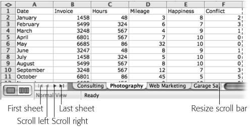
Scrolling through sheet tabs. If you have more sheet tabs than Excel can display in the bottom portion of the window, you can use the four tab scrolling buttons to scoot between the various sheets (see Figure 14-1). Another method is to Control-click any tab-scrolling button and then choose a sheet’s name from the contextual menu.
Showing more or fewer sheet tabs. The area reserved for Sheet tabs has to share space with the horizontal scroll bar. Fortunately, you can change how much area is devoted to showing sheet tabs by dragging the small, gray, vertical tab that sits between the tabs and the scroll bar. Drag it to the left to expand the scroll bar area (and hide worksheet tabs if necessary); drag it to the right to reveal more tabs.
Figure 14-1. The sheet scrolling buttons become active only when you become so fond of sheets that you can no longer see all their tabs at once. (Or maybe you just have a 12-inch PowerBook.) From left to right, the four sheet scrolling buttons perform the following functions: scroll the tabs to the leftmost tab, scroll the tabs to the left by one tab, scroll the tabs to the right by one tab, and scroll the tabs all the way to the right. Control-click any of the buttons and choose the sheet to go to from the pop-up menu. You can also make room for more tabs beneath your spreadsheet by dragging the left end of the lower scroll bar.
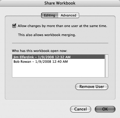
With a little preparation, several Excel fans on the same network can work on a single worksheet at the same time. (If you want to share a workbook, but prevent others from accessing it, read about protection on Protecting the spreadsheet first. Bear in mind, some protection commands have to be applied before you turn on sharing.) To share a workbook, choose Tools → Share Workbook, which brings up the Share Workbook dialog box. On the Editing tab (Figure 14-2), turn on “Allow changes by more than one user at the same time.” Click the Advanced tab for the following options:
Track changes. This section lets you set a time limit on what changes are tracked (see "Tracking Changes” on Tracking Changes). If you don’t care what was changed months ago, you can limit the tracked changes to 60 days. You can also tell Excel not to keep a change history at all.
Update changes. Here, you specify when your view of the shared workbook gets updated to reflect changes that others have made. You can set it to display the changes that have been made every time you save the file, or you can command it to update at a specified time interval.
If you choose to have the changes updated automatically after a time interval, you can set the workbook to save automatically (thus sending your changes out to co-workers sharing the workbook) and to display others’ changes (thus receiving changes from your co-workers’ saves). Or you can set it not to save your changes, and just to show changes that others have made.
Figure 14-2. The Share Workbook dialog box reveals exactly who else is using a shared workbook. If you worry that one of your fellow network citizens is about to make ill-advised changes, click his name and then click Remove User. Your comrade is now ejected from the spreadsheet party. If he tries to save changes to the file, he’ll get an error message explaining the situation. Please note that there’s little security in shared workbooks. As you can see, two people are logged in and able to make changes from two different Macs at the same time. Of course, if you password protect the sheet before sharing it, you’ll achieve a basic, keeping-honest-people-honest level of security.
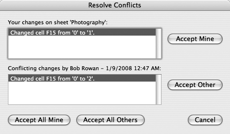
Conflicting changes between users. This section governs whose changes “win” when two or more people make changes to the same workbook cell. You can set it so that you’re asked to referee (which can be a lot of work), or so that the most recent changes saved are the ones that win (which can be risky). Clearly, neither option is perfect. Since each person can establish settings independently, it’s worth working out a unified collaboration policy with your co-workers (see Figure 14-3).
Include in personal view. These two checkboxes—Print settings and Filter settings—let you retain printing and filtering changes that are independent of the workbook. They can be set independently by anyone who opens the workbook.
When you click OK, Excel prompts you to save the workbook—if you haven’t already. Save it on a networked disk where others can see it. Now, anyone who opens the workbook from across the network opens it as a shared book.
Shared workbooks have some limitations, detailed in the Excel help topic, “Share a workbook.” Here’s a summary of things that you can’t do with a shared workbook:
Assign, change, or delete a password that protects a worksheet.
Insert charts, hyperlinks, objects, or pictures.
Make or change PivotTables, or make or refresh data tables (Step 2: Choose only the data you want).
Merge, insert, or delete blocks of cells; delete worksheets.
Use automatic subtotals or drawing tools.
Use or create conditional formats or data validation (Outlining).
View or edit scenarios (Scenarios).
Fortunately, there’s no need to give everyone on the network unfettered access to your carefully designed spreadsheet. You can protect your spreadsheet in several ways, as described here, and your colleagues can’t turn off these protections without choosing Tools → Unprotect Sheet (or Unprotect Workbook)—and that requires a password (if you’ve set one up).
Protect a workbook from changes. Choose Tools → Protection → Protect Workbook, which brings up the Protect Workbook dialog box. By turning on Structure and/or Windows, you can protect the workbook’s structure (which keeps its sheets from being deleted, changed, hidden, or renamed) and its windows (which keeps the workbook’s windows from being moved, resized, or hidden). Both of these safeguards are especially important in a spreadsheet you’ve carefully set up for onscreen reviewing. You can also assign a password to the workbook so that if someone wants to turn off its protection, he needs to know the password.
Protect a sheet from changes. Choose Tools → Protection → Protect Sheet to bring up the Protect Sheet dialog box. Turn on the Contents checkbox to protect all locked cells in a worksheet (described next). Turn on Objects to prevent changes to graphic objects on a worksheet, including formats of all charts and comments. Finally, turn on the Scenarios checkbox to keep scenario definitions (Scenarios) from being changed.
The bottom of the dialog box lets you assign a password to the worksheet; this password will be required from anyone who attempts to turn off the protections you’ve established.
Protect individual cells from changes. Excel automatically formats all cells in a new worksheet as locked, so if you protect the contents of a sheet you’ve been working in, all the cells will be rendered unchangeable. If you want some cells in a protected sheet to be editable, you have to unlock them while the sheet is unprotected. Unlock selected cells by choosing Format → Cells. In the resulting dialog box, click the Protection tab, turn off the Locked checkbox, and then click OK.
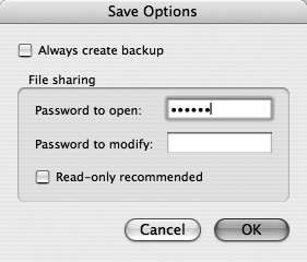
Require a password to open a workbook. Open the workbook you want to protect and choose File → Save As (or, if you’ve never saved this workbook before, choose File → Save). In the Save dialog box, click Options. In the resulting dialog box (Figure 14-4), enter one password to allow the file to be opened and, if you desire, another to allow file modification.
Tip
Alternatively, choose Excel → Preferences → Security and assign a password to open or to modify the workbook, and use the two buttons to access the Protect Workbook dialog box and the Protect Sheet dialog box.
Hide rows, columns, or sheets. Once you’ve hidden some rows, columns, or sheets (Hiding and showing rows and columns), you can prevent people from making them reappear by choosing Tools → Protection → Protect Workbook. Turn on Structure and then click OK.
Protecting a shared workbook. To protect a shared workbook, choose Tools → Protection → Protect Shared Workbook, which brings up the Protect Shared Workbook window. This window presents you with two protection choices. If you turn on "Sharing with track changes” and enter a password, you prevent others from turning off change tracking—a way of looking at who makes what changes to your workbook. Turning on this checkbox also shares the workbook, as detailed previously.
When people make changes to your spreadsheet over the network, you aren’t necessarily condemned to a life of frustration and chaos, even though numbers that you input originally may be changed beyond recognition. Exactly as in Word, Excel has a change tracking feature that lets you see exactly which of your co-workers made what changes to your spreadsheet and, on a case-by-case basis, approve or eliminate them. (The changes, not the co-workers.)
To see who’s been tiptoeing through your workbook, choose Tools → Track Changes → Highlight Changes, which brings up the Highlight Changes dialog box (Figure 14-5). In it, you can choose how changes are highlighted: by time or by the person making the changes. To limit the revision tracking to a specific area on the worksheet, click the spreadsheet icon at the right of the Where field, select the area, and then click the icon again.
As life goes on with this spreadsheet on your network, Excel highlights changes made by your co-workers with a triangular flag at the upper-left corner of a cell or block of cells (Figure 14-5, middle).
Once you’ve reviewed the changes, you may decide that the original figures were superior to those in the changed version. At this point, Excel gives you the opportunity to analyze each change. If you think the change was an improvement, you can accept it, making it part of the spreadsheet from now on. If not, you can reject the change, restoring the cell contents to whatever was there before your network comrades asserted themselves.
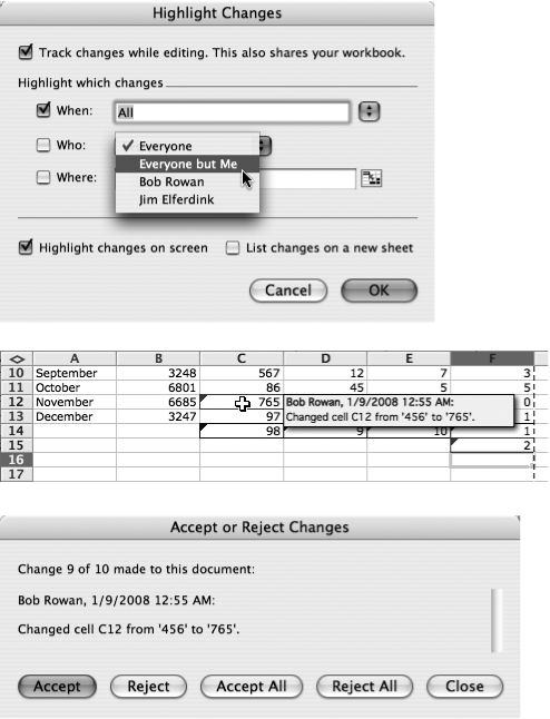
Figure 14-5. Top: This dialog box lets you turn on change tracking and specify whose changes are highlighted. By turning on Where, clicking the tiny spreadsheet icon next to the box, and dragging in your worksheet, you can also limit the tracking feature to a specific area of the worksheet. Middle: The shaded triangle in the upper-left corner of a cell indicates that somebody changed its contents. A comment balloon lets you know exactly what the change was. Bottom: Using this dialog box, you can walk through all the changes in a spreadsheet one at a time, giving each changed cell your approval or restoring it to its original value.
To perform this accept/reject routine, choose Tools → Track Changes → Accept or Reject Changes. In the Select Changes to Accept or Reject dialog box, you can set up the reviewing process by specifying which changes you want to review (according to when they were made, who made them, and where they’re located in the worksheet). When you click OK, the reviewing process begins (Figure 14-5, bottom).
In many work situations, you may find it useful to distribute copies of a workbook to several people for their perusal and then incorporate their changes into a single workbook.
Performing this feat, however, requires some preparation—namely, creating a shared workbook (see the previous section), and then configuring the workbook’s change history. You’ll find this option by choosing Tools → Share Workbook and then clicking the Advanced tab (Figure 14-6). The number that you specify in the “Keep change history for” box determines how old changes can be before they become irrelevant. The theory behind this feature contends that you’ll stop caring about changes that are older than the number of days that you set. (Tracking changes forever can bloat a file’s size, too.)
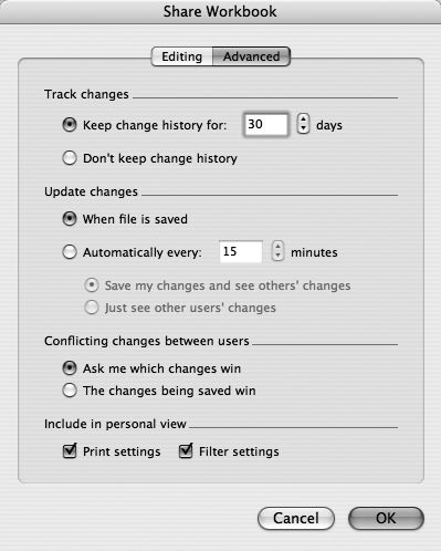
Figure 14-6. To prep your workbook for later merging, turn on the “Keep change history” option in the Share Workbook dialog box. You also have to complete your merge within the time limit that you set in the “Track changes” area. Once you’re ready to bring everything together, choose Tools → Merge Workbooks and select the first workbook that you want to merge into the current workbook.
Once you’ve prepared your workbook, distribute it via email or network. Ask your colleagues to make comments and changes and then return their spreadsheet copies to you (within the time limit you specified, as described in the previous paragraph). Collect all of the copies into one place. (You may need to rename the workbooks to avoid replacing one with another, since they can’t occupy the same folder if they have the same names.)
Now open a copy of the shared workbook and choose Tools → Merge Workbooks, which brings up an Open dialog box. Choose the file you want to merge into the open workbook, and then click OK. This process has to be repeated for every workbook you want to merge.
Every now and then, you may find it useful to send your Excel data to a different program—a database program, for example, or even AppleWorks (if you’re collaborating with somebody who doesn’t have Office). Fortunately, Microsoft engineers have built in many different file formats for your Excel conversion pleasure.
To save your Excel file in another file format, choose File → Save As; then select the file format you want from the Format pop-up menu. Here are a few of the most useful options in that pop-up menu.
If you’re sharing your document with Excel fans who have yet to upgrade to Excel 2008 for the Mac or Excel 2007 for PC (or if you’re uncertain), be sure and save your spreadsheet in this.xls format. The new (.xlsx) file format can only be read by Excel 2008 and 2007. (See page xxviii for more on the new XML file formats.)
The comma-separated file format is a popular way of getting your Excel sheets into other spreadsheets or databases (AppleWorks, FileMaker, non-Microsoft word processors, and so on). It saves the data as a text file, in which cell contents are separated by commas, and a new row of data is denoted by a “press” of the Return key.
Saving a file as a comma-separated text file saves only the currently active worksheet, and dumps any formatting or graphics.
Like comma-separated values, the tab-delimited file format provides another common way of getting your Excel sheets into other spreadsheets or databases. It saves the data as a text file, in which cell contents are separated by a “press” of the Tab key, and a new row of data is denoted by a “press” of the Return key.
Saving a file as a tab-delimited text file saves only the currently active worksheet, and dumps any formatting or graphics.
The Template file format is a special kind of Excel file that works like a stationery document: When you open a template, Excel automatically creates and opens a copy of the template, complete with all of the formatting, formulas, and data that were in the original template. If you use the same kind of document over and over, templates are an awesome timesaver. (For more on Excel templates, see Opening a Spreadsheet.)
To save an Excel workbook as a template, choose File → Save As and then select Template in the pop-up menu of the Save window. Excel proposes storing your new template in the Home → Library → Application Support → Microsoft → Office → User Templates → My Templates folder on your hard drive. Any templates you create this way appear in the My Templates portion of the Project Gallery and in the My Templates portion of the Sheets tab of the Elements Gallery (see Opening a Spreadsheet).
Where would a modern software program be without the ability to turn its files into Web pages?
Sure enough, Excel can save workbooks as Web pages, complete with charts, and with all sheets intact. In the process, Excel generates the necessary HTML and XML files and converts your graphics into Web-friendly file formats (such as GIF). All you have to do is upload the saved files to a Web server to make them available to the entire Internet. Once you’ve posted them on the Internet, others can look through your worksheets with nothing but a Web browser, ideal for posting your numbers for others to review. That’s the only thing they can do, in fact, since the cells in your worksheet aren’t editable.
To save a workbook as a Web page, choose File → Save as Web Page. At this point, the bottom of the Save window gives you some powerful settings that control the Web-page creation process:
Workbook, Sheet, Selection. Using these buttons, specify how much of your workbook should be saved as a Web page—the whole workbook, the currently active sheet, or just the selected cells. (If you choose Workbook, all of the sheets in your workbook will be saved as linked HTML files; there’ll be a series of links along the bottom that look just like your sheet tabs in Excel. Here again, though, these features won’t work smoothly for everyone, because not all Web browsers understand JavaScript and frames, which these bottom-of-the-window tabs require.)
Automate. This button brings up the Automate window, which lets you turn on a remarkable and powerful feature: Every time you save changes to your Excel document, or according to an exact schedule that you specify, Excel can save changes to the Web-based version automatically. Of course, you’ll still be responsible for posting the HTML and graphics files to your Web server.
To set up a schedule, click “According to a set schedule” and then click Set Schedule. In the Recurring Schedule window, set the Web version to be updated daily, weekly, monthly, or yearly. You can also specify the day of the week, as well as a start and end date for automatic updating. Updating happens only when the workbook is opened in Excel.
Web Options. The Web Options dialog box lets you assign appropriate titles and keywords to your Web pages. (The title appears in the title bar of your visitors’ browser windows and in search results from search engines like Yahoo and Google; search engines also sometimes reference these keywords.)
On the Pictures tab, you can also turn on PNG (Portable Network Graphics) graphics, which makes smaller graphics that download more quickly.
Excel gives you the chance to attach additional information to your files through something called properties. To call up the Properties dialog box for a worksheet, select File → Properties. In the resulting dialog box, you’ll see five tabbed subject areas with all kinds of information about your file:
General. This subject area tells you the document type, its location, size, when it was created and last modified, and whether it’s read-only or hidden.
Summary. This feature lets you enter a title, subject, author, manager, company, category, keywords, comments, and a hyperlink base for your document (the path you want to use for all the hyperlinks you create in the document).
Statistics. This tab shows when a document was created, modified, and last printed, as well as who last saved it. It also displays a revision number and the total editing time on the document.
Contents. Here, you’ll see the workbook’s contents—all of its sheets, even the hidden ones.
Custom. Finally, this tabbed area lets you enter any number of other properties to your workbook by giving the property a name, type, and value. You can enter just about anything here.