15.3 Synthetic Image Experiments

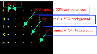
The synthetic image has the five mineral spectral signatures, A, B, C, K, M, marked by circles in Figure 1.12(b) are used to simulate 25 panels shown in Figure 15.1 with five panels in each row simulated by the same mineral signature and five panels in each column having the same size. Among 25 panels are five pure-pixel panels for each row in the first column and five pure-pixel panels for each row in the second column, the five -mixed pixel panels for each row in the third column and both the five subpixel panels for each row in the fourth column and the fifth column where the mixed and subpanel pixels are simulated according to legends in Figure 15.1. So, a total of 100 pure pixels (80 in the first column and 20 in second column), referred to as endmember pixels are simulated in the data by the five endmembers, A, B, C, K, M.

Figure 15.1 A set of 25 panels simulated by A, B, C, K, M.

These 25 panels are then inserted in a synthetic image with size of pixels in two ways. One is the background pixels removed to accommodate the inserted target pixels that result in target implantation (TI). The other is the inserted target panels directly superimposed over the background pixels that result in target embededness (TE). In both cases the background is simulated by the sample mean of the real image scene in Figure 1.12(a). Depending upon how a Gaussian noise is added to the TI and TE, three scenarios for each case are also simulated with details descried in Section 4.3. The goal of synthetic image experiments presented in this section is to study the role that kernelization plays in LSMA for hyperspectral imagery as well as its impact on unmixing performance. The six scenarios described in Chapter 4, TI1, TE2, TI3 and TE1, TE2, TE3 are simulated by the information provided in Figure 15.1 for performance evaluation.

Since all six scenarios produced similar results only the results for TE3 is selected as a representative example for illustration. Figure 15.2 shows the unmixed results of 130 panel pixels in TE 3 by LSOSP, NCLS, FCLS, and their kernel counterparts with RBF kernels used to perform kernelization where a Gaussian noise with SNR 20:1 is added to the target panel pixels which are directly superimposed over the background pixels.

Figure 15.2 LSMA and K-LSMA resulting image of synthetic linear mixture experiments.

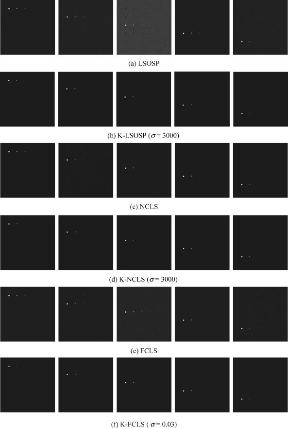
Through visual inspection of the results in Figure 15.1 only KLSOSP could slightly improve the detection of the panel pixels in the third row compared to its counterpart without using kernelization. Other than that it seemed that LSMA was not really benefited from kernelization in the sense of unmixing. To further support this conclusion, a 3D ROC analysis developed in Chapter 3 was performed on the unmixed results in Figures 15.2 and 15.3 show a 3D ROC curves of (P_D,P_F,τ), 2D ROC curves of (P_D,P_F), 2D ROC curves of (P_D,τ), and 2D ROC curves of (P_F,τ) where it was surprising to observe that the best results were not those produced by using kernelization.

Figure 15.3 3D ROC analysis of TE3 scenario, (a) 3D ROC curves of (P_D,P_F,τ); (b) 2D ROC curves of (P_D,P_F); (c) 2D ROC curves of (P_D,τ); (d) 2D ROC curves of (P_F,τ).

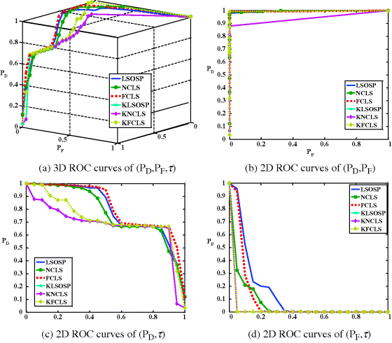
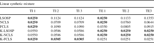
To see the whole picture of performance analysis conducted for six scenarios, Tables 15.1–15.3 tabulate the averaged detection rates of 130 panel pixels over the six scenarios resulting from 3D ROC analysis where the results indeed confirmed that the best results were those produced by LSMA shown in Tables 15.1 and 15.2 in terms of areas under the 2D ROC curves of (P_D,P_F) and 2D ROC curves of (P_D,τ). According to the areas of 2D ROC curves of (P_F,τ) in Table 15.3 kernelization did help LSMA reduce false alarm rates.

Table 15.1 Areas under 2D ROC curves of P_D versus P_F for TI and TE.

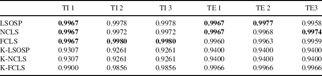
Table 15.2 Areas under 2D ROC curves of (P_D vs. τ) for TI and TE.

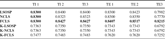
Table 15.3 Areas under 2D ROC curves of (P_F vs. τ) for TI and TE.

The above synthetic image experiments demonstrate an important fact that kernelization did not necessarily improve LSMA performance as we expected when the target pixels of interest were only lightly mixed in which case FCLS was always preferred to any other LSMA techniques regardless whether or not they were kernelized. This conclusion is further supported by the following experiments using two real data sets, AVIRIS Purdue data where data sample vectors are generally heavily mixed and HYDICE data where data sample vectors are less mixed.