31.2 Band Dimensionality Expansion
As shown in Chang and Brumbley (1999a, 1999b), the performance of OSP was considerably degraded if it was used for multispectral image classification due to an insufficient number of spectral bands to be used for orthogonal subspace projection. In order to address this issue, a recent effort in extending OSP to multispectral imagery was investigated by Ren and Chang (2000a) where an extended version of OSP, called Generalized OSP (GOSP), was developed by including a new technique, referred to as BGP, which allows users to expand spectral band dimensionality via nonlinear functions.
31.2.1 Rationale for Developing BDE
The idea of the BGP developed in Ren and Chang (2000a) arises from a second-order random process specified by the first-order and second-order statistics. If we view the original spectral bands image as the first-order statistical images, we can generate a set of second-order statistical spectral bands that capture correlation between spectral bands. These correlated images provide useful second-order statistical information among bands, which is missing in the set of the original spectral bands. The desired second-order statistics including auto-correlation, cross-correlation, and nonlinear correlation can be used to create nonlinearly correlated images. If there is a need of statistics of high orders, the same process can be carried out for this purpose. The concept of producing second-order or high-order correlated spectral bands coincides with moment generating functions used to generate various orders of moments for a random process. Despite that such a BDE may not have real physical meaning; it does provide a significant advantage to cope with the issue of the insufficient number of spectral band images. To shed light on this idea, we consider the following two examples.
As the first example, a farmer would like to give his own 17 cows to his three sons according to proportions of 17 cows, 1/2, 1/3, and 1/9. Obviously, there is no way to do so by simple arithemitics. However, if we introduce one hypothetic cow into 17 cows to make up a total of 18 cows, the problem is the well-solved because 1/2, 1/3, and 1/9 of 18 cows are 9 cows, 6 cows, and 2 cows, which are summed up exactly 17 cows. This simple example illustrates the idea of introduction of new band images by the BEP.
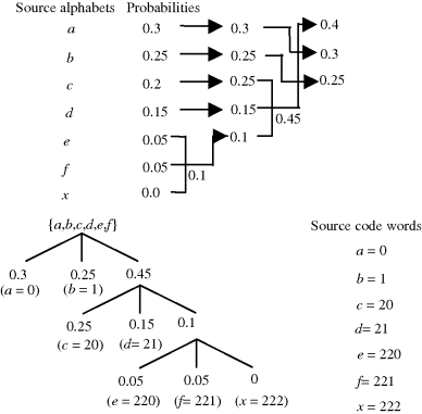
Another good example, which is more technical, is ternary Huffman coding from information theory. Assume that there is an information source X with six source alphabets {a,b,c,d,e,f} specified by their respective probabilities given by ![]() . The source entropy is
. The source entropy is
Suppose that these source alphabets are encoded by three source code word alphabets denoted by ![]() . What is the optimal Huffman code for {a,b,c,d,e,f}? Since the number of source alphabets is even, there is an unused node in a ternary Huffman coding tree. The best way is to leave this unused node as a leave rather than an internal node so that this unused node will produce the longest codeword as shown in Figure 31.1 rather than at the first internal node with shortest coding length shown in Figure 31.2.
. What is the optimal Huffman code for {a,b,c,d,e,f}? Since the number of source alphabets is even, there is an unused node in a ternary Huffman coding tree. The best way is to leave this unused node as a leave rather than an internal node so that this unused node will produce the longest codeword as shown in Figure 31.1 rather than at the first internal node with shortest coding length shown in Figure 31.2.
Figure 31.1 Huffman coding with an introduced dummy source alphabet x.

Figure 31.2 Huffman coding without introducing a dummy source alphabet x.

To achieve the desired code in Figure 31.1, we create a hypothetic source alphabet by introducing a dummy source alphabet x in Figure 31.1 so that this dummy alphabet x will be treated as a source alphabet with zero probability, thus it will have longest source code word, which does not exist. This idea is similar to the previous cow example described above where a hypothetic cow was introduced to make 17 cows a total of 18 cows so that the various proportions can be calculated based on the 18 cows. In the end such introduced hypothetic cow or dummy alphabet only serves as part of calculation but will not be counted for real.
31.2.2 Band Expansion Process
BEP presented in this section is essentially the same as BGP. It is renamed to reflect more accurately what the process does. Nevertheless, these two terminologies can be used interchangeably.
Let ![]() be the set of all original spectral band images. The first set of second-order-statistics spectral band images is generated based on autocorrelation. They are constructed by multiplying each individual spectral band image by itself, that is,
be the set of all original spectral band images. The first set of second-order-statistics spectral band images is generated based on autocorrelation. They are constructed by multiplying each individual spectral band image by itself, that is, ![]() . A second set of second-order-statistical spectral band images are made up of all cross-correlated spectral band images, which are produced by correlating any pair of two different spectral band images, that is,
. A second set of second-order-statistical spectral band images are made up of all cross-correlated spectral band images, which are produced by correlating any pair of two different spectral band images, that is, ![]() . Adding these two sets of second-order-statistics spectral band images to
. Adding these two sets of second-order-statistics spectral band images to ![]() produces a total of
produces a total of ![]() spectral band images. If more spectral band images are needed, other nonlinear functions may also be used to generate the so-called nonlinear correlated spectral band images. For example, we calculate third-order, fourth-order auto- or cross-correlated spectral band images or use a square-root function to produce
spectral band images. If more spectral band images are needed, other nonlinear functions may also be used to generate the so-called nonlinear correlated spectral band images. For example, we calculate third-order, fourth-order auto- or cross-correlated spectral band images or use a square-root function to produce ![]() or a logarithm function to produce
or a logarithm function to produce ![]() to stretch out lower gray level values. In what follows, we describe several ways to generate second-order, third-order, fourth-order auto- and cross-correlated spectral band images and some nonlinear correlated spectral band images.
to stretch out lower gray level values. In what follows, we describe several ways to generate second-order, third-order, fourth-order auto- and cross-correlated spectral band images and some nonlinear correlated spectral band images.
Algorithm for Band Expansion Process
It is worth noting that all the spectral band images generated by BEP are produced nonlinearly. These spectral band images should offer useful information for data analysis because they provide useful nonlinear spectral information to help to improve performance. However, we should point out that according to our experience, using the cross-correlated spectral band images generated by Step 2(ii) is generally sufficient to accommodate the need of BEP. Additionally, using the set of auto-correlated spectral band images produced by Step 2(i) may sometimes cause nonsingularity problems in matrix computation because they are self-correlated and usually very close to the original spectral band images. It is suggested that they should not be used alone and can only be used in conjunction with cross-correlated spectral band images. This can be well explained by the fact that a covariance matrix including variances and co-variances provides more information than a diagonal matrix, which only includes variances.
