33.4 Anomaly Detection

Anomaly detection received little interest in early days in remote sensing. There are several reasons attributed to this incident. One is due to applications which are mainly focused on geographic information processing such as land cover/use classification. Another is the use of multispectral imagery which has very low spatial and spectral resolutions. As a consequence, anomalies may be very much likely either embedded or mixed with other material substances in a single pixel vector. Under such circumstances, anomalies may have been contaminated or smeared by other dominant substances. Third, most remote sensing image processing techniques developed for such applications are spatial domain-based methods which are designed to take advantage of spatial correlation to perform image analysis. Since anomalies usually appear in a very limited spatial extent, such spatial domain-based methods can hardly capture their existence. Finally, anomalies do not provide much information to multispectral image analysts who are more interested in geographic information rather than target information. However, the advances of hyperspectral imaging sensors have revolutionized the way to process multispectral imagery. Due to the very high spectral resolution provided by hyperspectral sensors, many subtle substances that are generally unknown a priori or cannot be identified by visual assessment can now be uncovered for data analysis. On many occasions such substances are most interesting targets and provide crucial and critical information that can assist image analysts to solve many problems which cannot be resolved by multispectral imaging processing analysis. These applications may include agriculture, ecology, geology, environmental monitoring, law enforcement, military, and medical diagnosis. For example, subtle targets of interest can be special species in agriculture, unusual migrations in ecology, rare minerals in geology, toxic wastes in environments, drug trafficker or smugglers in law enforcement, vehicles/tanks in battlefields, cancerous cells or tumors in medical diagnosis, etc., just name a few. Such target signal sources generally appear in a form of abnormalities that are distinct from their surroundings. Therefore, how to characterize these types of target signal sources becomes crucial in image analysis. Three features can be suggested to characterize these target signal sources as anomalies: (1) existence, (2) presence, and (3) population. The reason of being anomalies is because they are not known a priori. On the other hand, anomalies usually occur with low probabilities. Therefore, their existence generally cannot be detected by any supervised means or visual inspection. As for presence, the spatial extent of anomalies is generally overlooked since they can be present as subpixel targets with their size smaller than pixel size or as mixed pixels mixing with the background or other substances. Most importantly, once anomalies do appear, their population cannot be large due to the nature of being anomalies. As a result, anomalies are generally considered as insignificant targets compared to the entire data. Unfortunately, several issues arising in anomalies have not been investigated or explored in the past. First, how large is it for a target to be considered as an anomaly in terms of its size? Second, how much spectral distinction is it for an anomaly to respond to its surrounding neighborhood? Third, how much sensitivity is it for an anomaly to noise? Fourth, how effective is it for an anomaly to distinguish itself from other anomalies? In particular, if two or more anomalies are close together, how can these anomalies be detected as separate anomalies? Finally, how can these anomalies be detected effectively by taking into account all the above-mentioned issues?

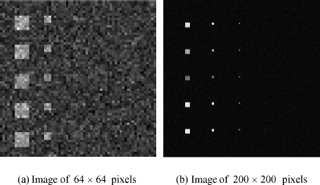
Many algorithms have been developed for anomaly detection over the past years and can be roughly categorized into two classes, second-order statistics methods and high-order statistics methods in terms of spectral statistics among data sample vectors. The detectors in the first class can be considered as either Mahalanobis distance-based filters which are variants of an algorithm developed by Reed and Yu (1990), referred to as RX detector (RXD) (Chang, 2003a) or matched filter-based detectors. The RXD-like detectors are primarily derived from generalized likelihood ratio test and adaptive subspace detectors via Gaussian noise assumption. One the other hand, the matched filter-based detectors do not make such assumption and simply makes use of the data sample spectral correlation matrix to whiten the sample data prior to implementation of a matched filter. Interestingly, the detectors of both types arrive at the same functional form due to the use of second-order statistics. The detectors in the second class take advantage of higher order statistics such as skewness (third order), kurtosis (fourth order), statistical independence (mutual information), or projection pursuit (relative entropy). It has been shown in Chang and Hsueh (2006) that when an early detected anomaly had a strong signature, it would affect detectability of follow-up anomalies, specifically for those anomalies with weak signatures. One way to mitigate this problem was to perform target discrimination once an anomaly was detected before searching for next anomalies. Such anomaly detection combined with target discrimination gives rise to anomaly classification (Chang and Chiang, 2002). However, in doing so, the process must be carried out in real time which cannot be implemented by most anomaly detection algorithms such as the RXD. The “real-time” referred here means that the pixel to be processed must be carried out in a causal manner that the pixels involved in data processing are only those that were already processed. To resolve this issue, a causal RX detector (CRXD) was further developed in to make the RXD a real-time processor. Recently, an adaptive anomaly detector, referred to dual window-based eigen separation transform (DWEST) was developed by Kwon et al. (2003) to address local properties of anomalies using an inner/outer window approach, and it was further investigated by a nested spatial window-based approach (Liu and Chang, 2004). These window-based adaptive anomaly detectors were designed to adapt local variability. However, some other issues such as size of anomalies, the response of anomalies to their surroundings, sensitivity of anomalies to noise, still remain and unsolved. One is of particular interest, “what is an anomaly?” In other words, what types of targets are considered as anomalies? A first attempt to address this issue was made in Chang and Hsueh (2006), which concluded that an anomaly should be closely related to its size relative to the image to be processed. The following simple example provides a clue of how controversial this issue is. Figure 33.5(a) and (b) shows a set of the same various target panels with four different sizes implanted in two simulated Gaussian noise-corrupted image backgrounds with sizes of 64 × 64 pixel vectors and 200 × 200 pixel vectors, respectively, where the five panels in the first column are size of 6 × 6 pixel vectors, the five panels in the second column are size of 3 × 3 pixel vectors, the five panels in the third column are size of 2 × 2 pixel vectors, and then the five panels in the fourth column are size of 1 × 1 pixel vectors.

Figure 33.5 Target panels with four various sizes implanted in two uniform image backgrounds with sizes of 64 × 64 pixel vectors and 200 × 200 pixel vectors.

The target implantation is done by replacing the background pixels with target panel pixels. Figure 33.6(a) and (b) shows the results of operating RXDF on these two images in Figure 33.5(a) and (b), respectively.

Figure 33.6 Results of operating RXD on images in Figure 33.3(a) and (b).

An immediate finding by comparing the results in Figure 33.6(b) to that in Figure 33.6(a) leads to an interesting observation: the target panels of sizes 2 × 2 and 1 × 1 that are detected by RXDF in Figure 33.6(b) as anomalies now become undetectable and are no longer anomalies in Figure 33.6(a) where two images in Figure 33.6(a) and (b) are shown in the same size for clear and better visual assessment. Moreover, the target panels of sizes 6 × 6 and 3 × 3 detected in Figure 33.6(a) also become smeared and blurred due to noise compared to their counterparts in Figure 33.6(b) which are detected clearly as anomalies. Why does the same RXDF produce so different results for the same set of target panels except that the processed image size is different? This simple example sheds light on a tricky issue in anomaly detection, “what does really it mean by anomaly?” Some answers can be found in the work by Chang and Hsueh (2006).

Despite the fact that many approaches described above have been developed for anomaly detection, an interesting approach to anomaly detection has been recently proposed by Liu and Chang (2008). It is called multiple-window anomaly detection (MWAD) which implements multiple a set of multiple windows to detect targets with varying sizes in order to avoid being trapped in the controversial definition of anomaly as demonstrated by the example presented in Figures 33.5 and 33.6. The idea is inspired by Figure 33.6(a) and (b), where the same target panels implanted in two different image sizes are detected by the same RXD in different abundance fractions. Since the size of the image to be processed must be fixed, it cannot be changed in the same way that is conducted in Figure 33.6 by the same RXD. To resolve this issue, the images processed in Figure 33.6(a) and (b) by RXD are now replaced by the images that are used to form the sample spectral correlation matrix for RXD to mimic two different image sizes. In other words, our proposed idea makes RXD adaptive to variable sizes of the sample covariance matrix used in RXD while keeping the original image size unchanged. More specifically, the sample covariance matrix used by RXD is formed by only image pixels within a designated window, in which case the window size determines the sample covariance matrix. Accordingly, adjusting the size of the sample covariance matrix used in RXD is similar to adjusting the original image size except that the sample covariance matrix used by RXD now varies with each image pixel vector that it processes. With this interpretation, the Reed-Yu's RXD can be viewed as a global anomaly detector where the entire image is considered as a single window to form the sample covariance matrix to capture the spectral variation provided by the entire image. More details about using various windows to perform anomaly detection are included in Chang (2013).

For many applications such as military/intelligence gathering or combat fields anomalies generally appear as moving targets. Therefore, developing real time processing algorithms for anomaly detection is highly desirable and critical. A detailed study on this subject can be found in Chang (2013).