4.4 Applications

The usefulness of the synthetic image-simulated six scenarios three applications are presented for illustration.

4.4.1 Endmember Extraction

Endmember extraction has received considerable interest in recent years and is probably one of the most important and crucial steps in hyperspectral image analysis since endmembers provide unique spectral information that is very valuable for data exploitation. Many algorithms have been developed and reported in the literature. Two most popular and widely used endmember extraction algorithms, pixel purity index (PPI) (Boardman, 1994) and N-finder algorithm (N-FINDR) (Winter, 1999a,b) with details in Chapter 7, were used for evaluation by the six designed scenarios. Since there are only five pure signatures, which are A, B, C, K, and M, dimensionality reduction required for PPI and N-FINDR was performed by the maximum noise fraction (MNF) transform (Green et al., 1998) to reduce the original data space to five dimensions. The results produced by the PPI using 500 skewers and N-FINDR are shown in Figures 4.10 and 4.11, respectively, where all pixels with PPI counts greater than zero are shown and marked by yellow pixels. Since there is no noise in TI1 and TE1, PCA instead of MNF was performed for dimensionality reduction.

Figure 4.10 Endmember extraction by PPI.

Figure 4.11 Five endmembers extracted by N-FINDR.

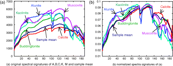
According to Figure 4.10, PPI was able to extract all five pure mineral signatures in all scenarios except TI1 and TE1. In particular, in TE1 PPI counts of all background pixels produced by the PPI were constant and greater than the PPI counts of the five pure mineral signatures because no noise was present in the data and the background dominates the entire data in which case it was considered as a pure signature. Similar results were also found by N-FINDR except one interesting finding which showed that N-FINDR could not extract the pure “calcite” signature in all TE scenarios. This is because the sample mean is used to simulate the image background and the signature of “calcite” is very close and similar to its signature in the sense of spectral similarity compared to other four mineral signatures. So, in this case, calcite was considered as a corrupted background signature so that once the background signature was extracted, the calcite could not be extracted. To see this, Figure 4.12 plots the spectral signatures of all the five minerals and the sample mean and their normalized spectral signatures to show the similarity among their spectral shapes where the sample mean in Figure 4.12(a) and the calcite have nearly the same shapes from band 1 to band 140 in Figure 4.12(b).

Figure 4.12 Spectra of A, B, C, K, M mineral signatures in the cuprite image scene and its sample mean signature.

The above experiments conducted based on Scenarios TI and TE also demonstrated several interesting results of how panel pixels extracted by PPI and N-FINDR in correspondence to five mineral signatures, which could not be observed by real image experiments. For example, N-FINDR successfully extracted all the panel pixels corresponding to five mineral signatures but in different manners where all the five extracted panel pixels in TI2 were from the first column compared to TI3 with two panel pixels from the first column and three panel pixels from the second column. A similar phenomenon was also observed in TE2 and TE3 except that N-FINDR successfully extracted the signature of calcite in TI2 and TI3 but failed to do so in Scenarios TE2 and TE3.

4.4.2 Linear Spectral Mixture Analysis (LSMA)

To perform LSMA, a linear mixing model is generally required where the complete target signature knowledge must be known a priori. It should be noted that in addition to the five endmembers discussed in Section 4.1, the background signature must be included in unmixing even when the background signature is mixed. This is because the background signature also represents a distinct spectral class in the data and cannot be excluded from being considered as an important signature to form the model. In this case, we assume that six distinct target signatures, which are five mineral signatures, A (alunite), B (buddingtonite), C (calcite), K (kaolinite), and M (muscovite) and a background signature, are the desired component signatures to be used to form a linear mixing model , where r is an image pixel, is the target signature matrix with the abundance vector specified by their corresponding abundance fractions , and n is a model correction term.

4.4.2.1 Mixed Pixel Classification

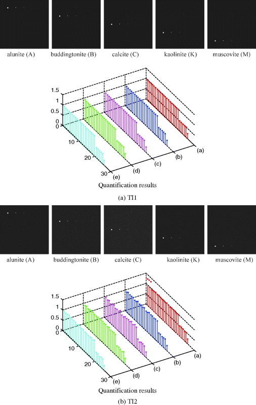
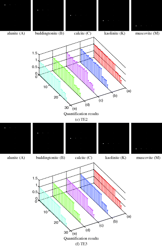
There are many mixed pixel classification methods available in the literature. One of the most widely used techniques is the so-called orthogonal subspace projection (OSP) developed by Harsanyi and Chang (1994) which has shown great success in various applications. Since OSP is developed as a signal detection technique and does not factor in abundance estimation, a least-squares OSP (LSOSP) was proposed by Tu et al. (1997) by including an abundance estimation error correction term in OSP as shown in Chang (1998). Figure 4.13 shows unmixed classification results by LSOSP along with their unmixed abundance fractions of each of the five mineral signatures where the labels of (a), (b), (c), (d), and (e) in quantification results corresponding to (A), (B), (C), (K), and (M) mineral signatures, respectively, and the LSOSP-unmixed abundance fractions were very close to true simulated abundance fractions for five mineral signatures.

4.4.2.2 Mixed Pixel Quantification

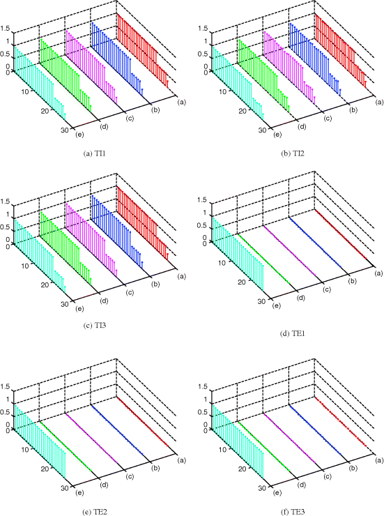
Despite that LSOSP has demonstrated its ability in unmixing abundance fractions as shown in Figure 4.13, it is an unconstrained spectral unmixing method which does not impose ASC and abundance nonnegativity constraint for . Consequently, the LSOSP-unmixed abundance fractions were not necessarily true fractions even though their unmixed fractions were more accurate than those produced by the OSP. So, for the purpose of mixed pixel quantification, these two constraints must be imposed on LSOSP. One such algorithm is the so-called FCLS method developed by Heinz and Chang (2001). Figures 4.14 graphically plot quantification results produced by FCLS for six scenarios where the labels of (a), (b), (c), (d), and (e) in quantification results corresponding to (A), (B), (C), (K), and (M) mineral signatures, respectively.

A very interesting and intriguing observation can be made from the results of three TE scenarios in Figure 4.14(c)–(f) where FCLS completely failed in quantifying all the five mineral signatures by throwing all abundance fractions to a single mineral signature, Muscovite. There is a reason for it. Since TE scenarios do not satisfy ASC, FCLS was forced to perform constrained quantification in which case it weighed all abundance fractions on the Muscovite due to the fact that the Muscovite has the most spectrally distinct signature among the five mineral signatures. This experiment demonstrated an important fact that constrained methods only worked effectively when the problems to be considered satisfy required constraints. These experiments further demonstrated the advantages of using synthetic images over real images.

Figure 4.14 FCLS-mixed pixel quantification results for six scenarios.

4.4.3 Target Detection

Unlike the mixed pixel classification/quantification which requires complete knowledge of target signatures assumed to be in the data, the target detection only needs a certain level of partial target knowledge. In this section two types of target detection are considered, subpixel target detection which only needs the knowledge of the target signature of interest and anomaly detection which does not need any target knowledge.

4.4.3.1 Subpixel Target Detection

One of the most powerful subpixel target techniques is the constrained energy minimization (CEM) developed by Harsanyi (1993). Its various forms have been investigated in Chang (2002b). CEM only assumes that the target of interest is given and designated as the desired target signature, d, while discarding all other knowledge including background knowledge. By specifying one of the five mineral signatures as a desired target signature, d, Figure 4.15 shows the detection results of panel pixels that were simulated by the particular signature d.

As we can see from the results in Figure 4.15, CEM also performed target detection very effectively including subpixel detection in the fourth and fifth columns. Most interestingly, CEM could detect small amounts of abundance fractions of other signatures simulated in mixed panel pixels, specifically panel pixels in the second row and the third column. Comparing the results in Figures 4.13 and 4.14, it can be clearly seen that LSMA made use of other signatures as unwanted signatures to suppress their interfering effects instead of detecting their abundance fractions as CEM did. Obviously, real image experiments cannot provide such evidence because there is no complete prior endmember knowledge for verification.

4.4.3.2 Anomaly Detection

When CEM is implemented, it requires the specific knowledge of the desire target signature of interest (Chang, 2003a). In many applications such as surveillance there is no prior knowledge regarding which targets we are looking for and which targets we are interested in. In this case, target detection must be performed without appealing for any prior knowledge. One widely used detection algorithm is developed by Reed and Yu (1990), referred to as RXD. Figure 4.16 shows the results of the six scenarios produced by RXD which detects all panel pixels in the first three columns but misses all the subpixel panels in the fourth and fifth columns.

Figure 4.16 Anomaly detection by RXD for six scenarios with an image size of pixel vectors.

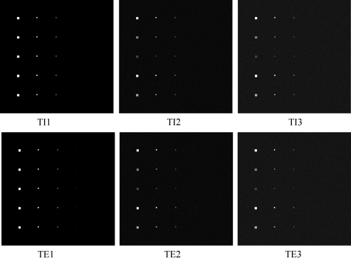
Now, if we operated RXD on the same six scenarios with a small image size of pixel vector where the same 25 panels simulated in Figure 4.2 were also inserted into these six scenarios with the image background, Figure 4.17 shows their RXD-detected results. An immediate finding by comparing the results in Figure 4.17 to those in Figure 4.16 led to an interesting observation. That is, the target panels of sizes and that were detected in TI2 and TE2 by RXD in Figure 4.16 as anomalies now became undetectable in TI2 and TE2 for RXD as shown in Figure 4.17, in which case they were no longer considered as anomalies in Figure 4.17. Moreover, the performance of operating RXD on scenarios of TI and TE in Figure 4.16 was nearly the same and so was for scenarios of TI3 and TE3 in Figure 4.16. But this was not the case for RXD operating on a smaller image scene with the same identical 25 panels in Figure 4.17 where RXD had complete opposite results for TI1 and TE1 and quite different results for TI3 and TE3. Why did the same RXD produce different results for the same set of 25 panels inserted into the same image background with the only difference in the size of the processed image scenes? This simple example sheds light on the utility of the designed six scenarios which shows a tricky issue in anomaly detection, “what is really meant by anomaly?”, a topic to be discussed in Chapter 18, Chang and Hsueh (2006) and Chang (2013).

Figure 4.17 Anomaly detection by RXD for six scenarios with an image size of pixel vectors.