33.3 Linear Spectral Mixture Analysis

Linear spectral mixture analysis (LSMA) is a theory developed for sub-sample and mixed sample analysis discussed in Chapter 2, whereas LSU is a technique to carry out LSMA to unmix data sample vectors via a linear mixing model into a number of basic constituent spectra assumed to make up the entire data sample vectors with appropriate abundance fractions of these constituent spectra. In spite of this distinction, these two terminologies have been used interchangeably in the literature. Depending on whether or not the signature knowledge is available, LSMA can be carried out by supervised LSMA (SLSMA) or ULSMA.

There are three crucial differences between LSMA and classification. One is that the spectral unmixing performed by LSMA produces abundance fractional maps considered as soft decisions as opposed to classification, which produces classification maps considered as hard decisions. Another difference is that LSMA only requires signature knowledge to form a linear mixture model and does not need training samples as required by classification. Even for ULSMA, the signature knowledge can be obtained by endmember extraction algorithms or unsupervised virtual signature finding algorithms (UVSFAs) developed in Chapter 17 where the only training samples are endmembers or virtual signatures themselves. So, the cross-validation used by classification via a set of training samples to evaluate performance is not applicable to LSMA. A third difference is background suppression. LSMA takes the advantage of OSP to eliminate effects of undesired signatures to improve background suppression so as to enhance unmixing ability of desired signals, a task that generally cannot be done by classification. Due to the lack of background knowledge such background suppression cannot be evaluated quantitatively but is better evaluated by visual assessment of each of abundance fractional maps. Nevertheless, the 3D ROC analysis developed in Chapter 3 can be further used as an evaluation tool to allow users to perform quantitative analysis and study of abundance fractional maps.

33.3.1 Supervised LSMA

Solving LSMA is a least squares estimation problem. It makes use of a linear mixing model specified by

(33.20)

where M is a signature matrix formed by a set of p known signatures, and n can be interpreted in various applications. When the n is considered as a model error, the solution to (33.20) is given by (12.24) as

(33.21)

which is the least squares estimation of the abundance vector α (Shimabukuro and Smith, 1991; Settle and Drake, 1993). On the other hand, if n is interpreted as a Gaussian noise in Section 12.3.3, the solution to (33.20) is the given by the Gaussian Maximum Likelihood (GML) estimator (Settle, 1996; Chang, 1998a) as

(33.22)

which is the MSE estimate of abundance vector α that is identical to (33.21).

As a completely different treatment, Harsanyi and Chang (1994) developed an OSP-based approach to LSMA form a signal detection point of view. Instead of considering (33.20) as an estimation problem by estimating abundance fractions of all endmembers all together as (33.21) and (3.22) the OSP idea considers the problem of (33.20) as a multiple signal detection problem for p signal sources present in the data where it makes use of signal-to-noise (SNR) as a criterion (also known as deflection criterion in detection theory) to measure signal detection performance. In this case, it only assumes that the noise is additive but not necessarily Gaussian. According to (33.20), the signal detection is carried out by considering Mα as a single signal source which is actually a mixed signal source linearly combining the p signal sources, . Thus, it does not discriminate multiple signal sources detected in the data. To resolve this issue, OSP extends the standard single-signal detection approach by a two-stage process to solve (33.20) as a multiple-signal detection problem. More specifically, Let be the desired signal source to be detected. Under this circumstance, all the remaining signal sources, p signal sources , will be considered as interferers to m_p which must be annihilated prior to detection of m_p so as to increase as well as enhance detectability of m_p. The key idea of OSP is to introduce an operator for this purpose to eliminate the influence of these p − 1 undesired signal sources prior to detection of the desired signal source m_p. In other words, let be an undesired signal source matrix. An operator defined by

(33.23)

maps all data sample vectors onto a space, , orthogonal to the space linearly spanned by the p − 1 signal sources . Taking advantage of operating on the model in (33.20) results in

(33.24)

where the undesired signatures in U have been annihilated and the original noise n has also been suppressed to . The role of plays in (33.24) is to remove all signal sources other than d from the mixed signal source Mα so that only the desired signal source d will be present in . In this case, the desired signal source will also be suppressed by as . As a consequence, (33.24) becomes a standard model commonly used in communications and signal processing to detect the single signal source . The optimal solution to (33.24) previously derived from (12.5) to (12.9) in Chapter 12 is a matched filter, M_d, given by

(33.25)

Two interpretations can be made on (33.25). One is to interpret OSP as a matched filter using the “d” as the desired matching signal source to extract d from all data sample vectors in the space . Alternatively, OSP can also be interpreted as a matched filter which a matched signal source “” to extract the desired signal source from data sample vector r in the original data space. Using (33.25) the abundance fraction of the desired signal source can be detected as

(33.26a)

where the constant κ is generally set to κ = 1 for the purpose of detection. Accordingly, for the OSP to perform multiple signal detection, two-stage processes can be designed in sequence as follows.

The first-stage process separates a desired signal source d from other signal sources which form an undesired signal source matrix U so that an undesired signal source annihilator is applied to all data sample vectors in the original data space to suppress the effects of the undesired signal sources on detection of the desired signal source d. This is then followed by the second-state process, which implements a matched filter to extract the desired signal source d. Such a two-stage process can be considered as an information-processed matched-filter which has been studied in great details in Chang (2007c). For example, since OSP assumes that the complete knowledge of signal sources, is known a priori, it can take advantage of and d to carry out two-stage processes in Figure 33.3. However, in many applications such knowledge may not be available. In this case, the a priori knowledge of and the desired signal source d must be replaced with the a posteriori knowledge R⁻¹ where R is the auto-correlation matrix formed by all data sample vectors and the data sample vector currently being processed r. As a result, becomes an anomaly detector, which is exactly so-called RX-detector developed by Reed and Yu (1990). On the other hand, the above two-stage process in Figure 33.3 can also be implemented as the one-shot operation process by linear constrained minimum variance (LCMV) filter developed by Chang (2002b) and Chang (2003a, Chapter 11) where the detection of d and annihilation of U are carried out simultaneously at the same time. Many more details can be also found in Chapter 12.

Figure 33.3 A block diagram of .

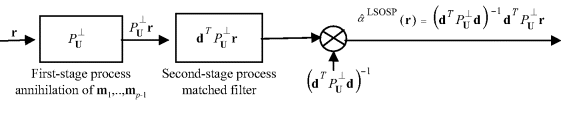
It has been shown in Settle (1996) and Chang (1998a) that the constant κ accounts for estimation accuracy and cannot be arbitrary if (33.26a) is used to estimate the abundance fraction of d = m_p in which case κ must be set by . When OSP implements (33.26a) by setting

(33.26b)

it is called LSOSP (Tu et al., 1997), which produces exactly the same abundance fraction estimated by (33.21) and (33.22) for the endmember m_p, where and are the pth component of the estimated abundance vectors and , respectively. The key difference between (33.26a) and, (33.21), and (33.22) is that the former only estimates the abundance fraction of one particular signal source m_p as opposed to the latter which estimates abundance fractions of all the p signal sources, simultaneously. In other words, the LSOSP basically makes a signal detector a signal estimator in terms of converting -detected abundance fraction to the -estimated abundance fraction.

Furthermore, replacing the constant κ in Figure 33.3 with results in Figure 33.4 depicted as follows.

Figure 33.4 A block diagram of .

As noted earlier, if the a priori knowledge of is not available, a posteriori knowledge R⁻¹ with R being the autocorrelation matrix formed by all data sample vectors can be used to replace . In this case, the in (33.26a) and Figure 33.4 becomes the given by (2.33) where the desired signal source d is identified by a target signal source of interest, t. Finally, it should be noted that the LSOSP, bridges the gap between the OSP detector, and LS estimator, . By virtue of LSOSP, the OSP can be further extended to abundance-constrained least squares methods, NCLS and FCLS methods discussed in Chapter 2 and Chang (2003a).

There are several approaches to extending SLSMA. It has been shown by Juang and Katagiri (1992) that the LSE resulting (33.20) is not an appropriate criterion for classification. It is also known that Fisher linear discriminant analysis is very effective in classification due to its use of Fisher's ratio particularly designed for class discrimination. So, one approach is to replace the LSE criterion used by LSMA with classification criterion, Fisher's ratio. The resulting LSMA is called Fisher's LSMA (FLSMA) discussed in Chapter 13. It turns out that the LSE used by LSMA becomes Fisher's ratio for FLSMA where S_W is the within-class scatter matrix defined in (13.1). Another is to generalize the LSE criterion to a weighted LSE criterion, denoted by where the weighting matrix A is a positive definite matrix. The resulting LSMA is called weighted abundance constrained LSMA (WACLSMA) discussed in Chapter 14. Consequently WACLSMA can be considered as a generalized LSMA which includes the standard LSMA and FLSMA as it special cases by setting A = identity matrix I and , respectively.

33.3.2 Unsupervised LSMA

While SLSMA has been well studied in the literature, ULSMA has not received as much attention as it should have due to the following reasons. To perform LSMA effectively, the accurate signature knowledge is required. In SLSMA, such knowledge is provided by a set of constituent spectra, , referred to as endmembers in the literature, which are known provided by either prior knowledge or visual inspection. However, according to the definition in Schowengerdt (1997), an endmember must be an idealized, pure signature for a class. Unfortunately, as reported in many recent results (Chang et al., 2006; Wu et al., 2009) this is generally not true for real datasets where a true endmember may never exist. Nevertheless, this does not prevent users from using the term of endmembers. To address this issue, the desired endmembers required by LSMA must be obtained directly from the data to be processed. However, this easier said than done because finding an appropriate set of for LSMA is very challenging and not a trivial matter with two issues involved. The first one is to determine how many signatures should be used by LSMA for spectral unmixing. The concept of VD developed in Chapter 5 is particularly designed to address this issue with extensive discussion in Section 33.1.1 where VD is defined as the number of spectrally distinct signatures, p in hyperspectral data instead of the number of endmembers. Once the value of the p is determined, the second and following issue is how to find these p signatures, . Obviously, each of represents one distinct spectral class and is not necessarily an endmember. Some of may be even mixed signatures. Accordingly, the term of endmembers commonly used in LSMA to represent these basic constituent spectra is misleading. A better terminology may be virtue endmembers (VEs) to reflect this fact that VEs represent spectrally distinct signatures in correspondence to the definition of VD. Because of that VD-estimated value is generally greater than the number of endmembers. In other words, the number of VEs, n_VE, is generally not the same as the number of endmembers, n_E. In this case, an endmember extraction algorithm may not be effective to extract all necessary VEs. The ULSMA presented in Chapter 17 is specifically developed to resolve issues of determining the value of p and finding a desired set of VEs, referred to as virtual signatures (VSs) to reflect that VSs are real pixels directly extracted in the data.