
31.6 Multispectral Image Experiments
The multispectral image data used for experiments is shown in Figure 31.7. The image scene was collected by the Satellite Pour l'Observation de la Terra (SPOT) system in three spectral bands, two of which are from visible region of electromagnetic spectrum, band 1: 0.5–0.59 μm and band 2: 0.61–0.68 μm and the third band is from near-infrared region of electromagnetic spectrum, 0.79–0.89 μm. The ground sampling distance is 20 m. The image scene has size 256 × 256 was taken over Northern Virginia where in the scene there are the Falls Church High School, the Little River Turnpike, a lake at the upper right corner and the Mill Creek Park.
Figure 31.7 Three spectral band images of SPOT data.

According to the ground truth obtained from visiting the site as well as provided by the Google Earth, there are at least four signatures, buildings, roads/parking lots, water, and vegetation in the scene with training samples selected from the four marked areas shown in Figure 31.8 to represent these four different classes. The signatures used to form the signature matrix M for LSMA were obtained by sample means of training samples from the four marked areas, that is, M = [mlake, mvegetation, mbuilding, mroads] where marea is the sample mean of the area.
Figure 31.8 Training samples selected from four areas in Northern Virginia.

To carry out BEP, two sets of BEP bands were used, autocorrelated bands and cross-correlated bands, where both autocorrelated bands and cross-correlated bands were normalized by their corresponding variances of spectral band images. Six experiments were conducted to evaluate the effectiveness of BEP and kernelization in conjunction with LSMA in performance analysis where LSMA, BEP6 + LSMA, BEP9 + LSMA, KLSMA, BEP6 + KLSMA, and BEP9 + KLSMA were used to perform spectral unmixing with BEP6 and BEP9 defined as

Experiment 31.1 (LSMA)
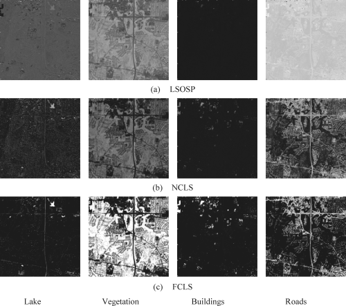
In this experiment three LSMA techniques, LSOSP, NCLS, and FCLS were operated on the three-band original SPOT data without nonlinear dimensionality expansion. Figure 31.9(a)–(c) shows the unmixed results of the SPOT data produced by LSOSP, NCLS, and FCLS, respectively, where FCLS obviously outperformed the other two, LSOSP and NCLS.
Figure 31.9 Unmixed results of SPOT data produced by (a) LSOSP, (b) NCLS, and (c) FCLS.

Experiment 31.2 (BEP6 + LSMA)
This experiment was conducted in the same way that Experiment 31.1 was performed except that LSOSP, NCLS, and FCLS were applied to BEP6 image data. Figure 31.10(a)–(c) shows the unmixed results produced by LSOSP, NCLS, and FCLS, respectively, where FCLS was still the best followed by NCLS as the second best with LSOISP being the worst. Compared to results shown in Figure 31.9, FCLS performed nearly the same with no obvious improvements, LSOSP was indeed slightly improved, but NCLS was improved drastically. This experiment shows that three LSMA-based techniques could be benefited from three extra cross-correlated spectral bands, which actually provided useful spectral information that could improve the unmixing ability.
Figure 31.10 Unmixed results of SPOT data produced by (a) LSOSP, (b) NCLS, and (c) FCLS with using BEP 6.
Experiment 31.3 (BEP9 + LSMA)
The only difference between this experiment and Experiment 31.2 was the data which included three more auto-correlated spectral bands in addition to the three cross-correlated spectral bands. Figure 31.11(a)–(c) shows the unmixed results produced by LSOSP, NCLS, and FCLS, respectively.
Figure 31.11 Unmixed results of SPOT data produced by (a) LSOSP, (b) NCLS, and (c) FCLS with using BEP 9.

Compared to the results in Figure 31.10, the improvement from BEP6 to BEP9 was very little and hardly recognized. This implies that including autocorrelated spectral bands did not really help much once cross-correlated spectral bands are used.
Experiment 31.4 (KLSMA)
This experiment was conducted to see how much improvement that LSMA could be benefited from kernelization where RBF kernel was used with three different values of σ selected empirically. Figures 31.12–31.14 show the unmixed results produced by KLSOSP, KNCLS, and KFCLS, respectively, where in all cases FCLS remained the best, but interestingly, LSOSP and NCLS performed very closely.
Figure 31.12 Unmixed results of SPOT data produced by KLSOSP with different values of σ.

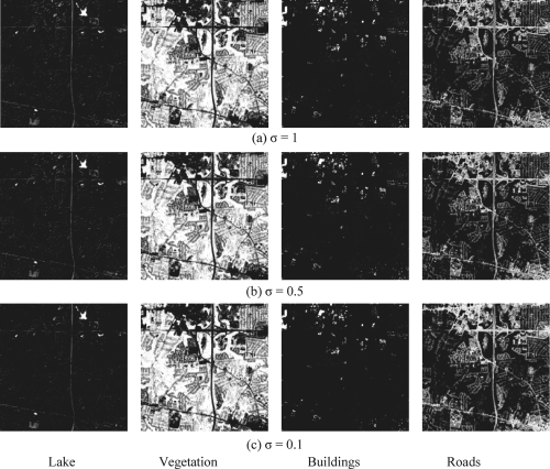
Figure 31.13 Unmixed results of SPOT data produced by KNCLS with different values of σ.
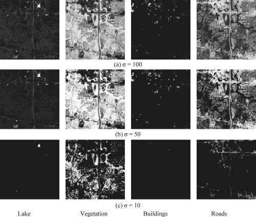
Figure 31.14 Unmixed results of SPOT data produced by KFCLS with different values of σ.

If we compare the results against their counterparts without kernelzation, the improvement resulting from kernelization was very significant, specifically, LSOSP.
In the previous four experiments, only one nonlinear dimensionality technique was implemented, either BEP or kernelization but not both. The following two experiments was performed to see whether or not unmixing ability can be further improved if both BEP and kernelization are used for nonlinear dimensionality expansion.
Experiment 31.5 (BEP6 + KLSMA)
This experiment implemented KLSMA on the image data produced by BEP6. Figures 31.15–31.17 show the unmixed results produced by KLSOSP, KNCLS, and KFCLS, respectively.
Figure 31.15 Unmixed results of SPOT data produced by KLSOSP using BEP6 with different values of σ.

Figure 31.16 Unmixed results of SPOT data produced by KNCLS using BEP6 with different values of σ.
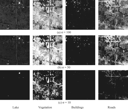
Figure 31.17 Unmixed results of SPOT data produced by KFCLS using BEP6 with different values of σ.

Compared to the results shown in Figs 31.12–31.14, the difference between “KLSMA without BEP” and “KLSMA with BEP6” was not very visible. In other words, the advantages provided by BEP seemed to vanish after kernelization. This indicated that kernelization is more effective than BEP when considering came spectral unmixing. This made sense because pixels in multispectral images are generally heavily mixed, and the pixel mixtures may not be linear either.
Experiment 31.6 (BEP9 + KLSMA)
This experiment was performed by taking both advantages, BEP9 and kernelization. Figures 31.18–31.20 show the unmixed results produced by KLSOSP, KNCLS, and KFCLS, respectively. As we can see by comparing the results to those in Experiment 31.5 BEP9 seemed not to provide any better benefit than BEP6 did, a similar phenomenon observed in Experiments 31.2 and 31.3 regardless of whether kernelization was used.
Figure 31.18 Unmixed results of SPOT data produced by KLSOSP using BEP9 with different values of σ.
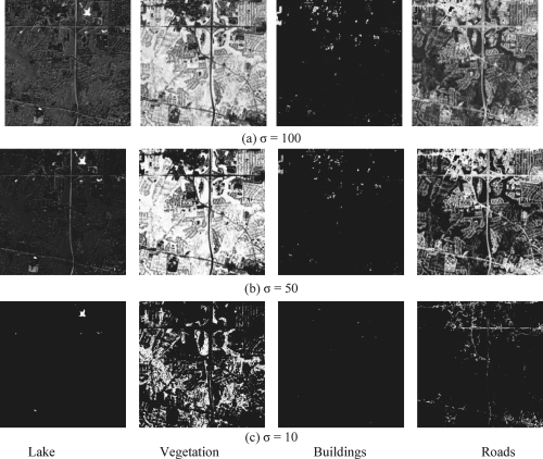
Figure 31.19 Unmixed results of SPOT data produced by KNCLS using BEP9 with different values of σ.

Figure 31.20 Unmixed results of SPOT data produced by KFCLS using BEP9 with different values of σ.
Based on the above six experiments, we can draw the following conclusions.
To conclude this section, it is worth mentioning that there is another application of applying BEP + LSMA and KLSMA to magnetic resonance (MR) image classification presented in the following chapter, Chapter 32. The superior performance of KLSMA to LSMA in quantitative analysis will be shown in this chapter and has been also demonstrated in Wong (2011) by experiments using synthetic magnetic resonance (MR) brain images provided by McGill University (http://www.bic.mni.mcgill.ca/brainweb/). Those who are interested in quantitative studies and analyses are encouraged to find details in this reference.