31.4 Feature Dimensionality Expansion by Nonlinear Kernels

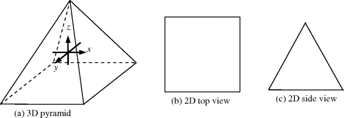
Unlike BDE, which expands band dimensionality to resolve the issue in use of an insufficient number of spectral bands, FDE makes a rather different attempt by expanding features used by classification to a high dimensional feature space via a nonlinear kernel so that the linear nonseparability issue arising in the original data space can be resolved in a new feature space. Its idea can be briefly illustrated by the following example. Assume that a three-dimensional (3D) pyramid shown in Figure 31.5(a) is viewed in a two-dimensional space. It must require two views, a 2D top view shown in Figure 31.5(b) and a 2D side view shown in Figure 31.5(c) to completely envision what a pyramid looks like in a 3D space.

Using the pyramid in Figure 31.4(a) as an example, solving a linear nonseparable problem in an original data space is similar to viewing a pyramid in a two-dimensional data space, which requires two different views, top and side views, to capture its shape, which can only be visualized in a three-dimensional space. This is equivalent to expanding two top and side views to a single view of a pyramid in a three-dimesnional space shown in Figure 31.4(a), which becomes linearly separable problem.

Figure 31.4 A three-dimensional pyramid can be viewed by jointly 2 two-dimensional top and side views.

Two kernel-based approaches are generally developed in the literature. One is FDE by transform, which utilizes a nonlinear kernel function to map a component analysis-based transformation such as PCA, ICA into a higher dimensional feature space so that nonlinear separable data features can be recognized by a linear classifier in this new feature space. The main hurdle of this approach is excessive computational complexity resulting from kernelization where all data sample vectors are considered as feature vectors to be kernelized. The second approach is FDE by classification, which only kernelizes the training sample vectors used to train classifiers such as SVM and FLDA. As a consequence, the issue of computational complexity caused by data sample vectors in FDE by transform is mitigated by computational complexity which is only involved with the training sample vectors. In what follows, these two approaches are presented in two separate subsections.

31.4.1 FDE by Transformation

Kernel-based approaches have found great success in many applications in the sense that feature vectors extracted from the original data space are nonlinearly transformed to a higher feature dimensional space to resolve the issue of linear nonseparable problems. This section presents a kernel version of the most widely used transformation, principal components analysis (PCA) developed by Scholkopf et al. (1999b).

For presenting, we reiterate the PCA described in Section. Assume that is a set of L-dimensional image pixel vectors, and μ is the mean of the sample pool S obtained by . Let X be the sample data matrix formed by . Then, the sample covariance matrix of the sample pool S can be calculated by . If we further assume that is the set of eigenvalues obtained from the covariance matrix K and are their corresponding unit eigenvectors, that is, , we can define a diagonal matrix D_σ with variances along the diagonal line as

(31.2)

and an eigenvector matrix Λ specified by as

(31.3)

such that

(31.4)

Using the eigenvector matrix Λ, a linear transform ξ_Λ defined by

(31.5)

transforms every data sample r_i to a new data sample, by

(31.6)

As a result, the mean of new ξ_Λ-transferred data samples becomes and its resulting covariance matrix is reduced to a diagonal matrix given by

(31.7)

Equation (31.7) implies that the ξ_Λ-transferred data matrix has been de-correlated or whitened by the matrix Λ, which is referred to as a whitening matrix (Poor, 1994). The transform ξ_Λ defined by (31.6) is generally called principal component transform and the lth component of is formed by

(31.8)

and is called the lth principal component (PC) which consists of that are -transferred data samples corresponding the lth eigenvalue λ_l. The PCA is a process that implements the transform ξ_Λ defined by (31.5) to obtain a set of PCs via (31.6) or (31.8) with all .

PCA is a process that implements the transform ξ_Λ defined by (31.5) to obtain a set of PCs via (31.6) or (31.8) with all . To achieve DR, only those PCs specified by eigenvectors that correspond to first q largest eigenvalues will be retained, while the PCs specified by eigenvectors corresponding to the remaining (L–q) smaller eigenvalues will be discarded. In what follows, we follow the approach proposed in Scholkopf et al. (1999b) to extend the PCA to the so-called Kernel PCA (K-PCA) via a nonlinear function.

Assume that the original data space X is made up of N L-dimensional data sample vectors , and ϕ is a nonlinear function which maps the data space X into a feature space F, with dimensionality yet to be determined by a kernel, that is,

(31.9)

We further assumed that the mapped data samples into the feature space are centered, that is, . Now we can define the sample covariance matrix in the feature space F by the

(31.10)

Using the same argument outlined by (31.1–31.5), let be the eigenvalues of specified by (31.10) and be their corresponding eigenvectors with unit length, that is, . Then,

(31.11)

Multiplying both sides of (31.11) by ϕ(r_k) results in

(31.12)

Since lies in the space linear spanned by the data samples in the space F, , it can expressed by

(31.13)

where is a combinitorial coefficient vector of . Substituting (31.10) and (31.13) into (31.12) yields

(31.14)

where

(31.15)

To find a solution to (31.14), we only need to solve

(31.16)

Using (31.16) and gives rise to

(31.17)

To find the lth principal component in the feature space F, we project all data samples ϕ(r) in F onto the lth eigenvector via the following equation:

(31.18)

It should be noted that to calculate (31.15) and (31.18), we only need to perform dot products without actually using explicit forms of the nonlinear function ϕ, which is referred to as kernel trick in Section 2.4.1.

31.4.2 FDE by Classification

Two types of FDE by classification are considered, one using sample spectral correlation and the other using intrapixel spectral correlation.

31.4.2.1 FDE by Classification using Sample Spectral Correlation

The FDE by classification using sample spectral correlation take advantage of spectral correlation among sample vectors to improve and enhance classification. This type of classifiers includes hard decision-made classifiers such as MLC and soft decision-made detectors, RXD and CEM, all of which include either sample spectral covariance matrix or sample spectral correlation matrix as additional spectral information to improve their performance in solving non-linear separable problems. Their kernel counterparts are referred to as kernel-based MLC (KMLC), kernel-based FLDA (K-FLDA), kernel-based RXD (KRXD), and kernel-based CEM (KCEM). Since the sample spectral covariance/correlation matrix used by this type of classifiers for FDE is formed by all the data sample vectors, its size determines computational complexity, which turns out to be the same issue encountered in FDE by transform. However, an advantage of these classifiers used for FDE over FDE by transform is that these classifiers can be made adaptive classifiers by considering various window sizes to capture local spectral correlation to replace the global sample spectral correlation. As a result, the number of the sample vectors embraced by a local window is only limited to the window size which can significantly ease computational complexity. The resulting classifiers are referred to as Kernel-based adaptive MLC (KAMLC), kernel-based adaptive RXD (KARXD), Kernel-based adaptive CEM (KACEM).

Two interesting facts are noteworthy.

31.4.2.2 FDE by Classification using Intrapixel Spectral Correlation

The FDE by classification using intrapixel spectral correlation has been discussed in Chapter 15 where three KLSMA-based classifiers, kernel-based orthogonal subspace projection (KOSP), kernel-based least-squares orthogonal subspace projection (KLSOSP), kernel-based non-negativity constrained least squares (KNCLS), and kernel-based fully constrained least squares (KFCLS) are derived. These classifiers make use of intrapixel spectral correlation provided by the signature matrix M in (2.78). Since these classifiers are operated on a single pixel vector basis, their kernel-based counterparts are determined by the number of signatures, p, used in the M not the data size and signatures used to unmix data sample vectors. Accordingly, the kernelization trick is actual performed on the classifiers themselves not on training samples or on data sample vectors. This type of FDE by classification is the third kernelization approach described in Section 15.2.4. As a consequence, their computational complexity is significantly reduced because the value of the p is very small compared to the data size. In this case, all the KLSMA classifiers developed in Chapter 15 are easy to implement.

Finally, Figure 31.5 summarizes two approaches to FDE where various transformations used in FDE by transform and various classifiers used by FDE by classifiers are described.

Figure 31.5 Feature dimensionality expansion techniques for multispectral imagery.