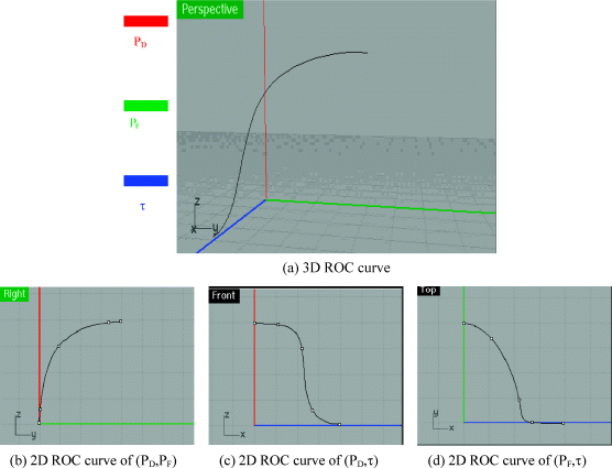
3.4 3D ROC Analysis
From the hypothesis testing problem specified by (3.1), a detector makes a binary hard decision by thresholding a real-valued LRT, Λ(r), via a threshold τ (see (3.5)). Accordingly, the detector performance is determined by two parameters, Λ(r) and τ, both of which are real values. As a result, the detection rate, PD, in (3.2) and (3.6) and the false alarm probability/rate PF in (3.3) and (3.7) are indeed functions of Λ(r) and threshold τ. However, in the Neyman–Pearson detection theory the cost function  and prior probabilities
  are assumed to be not known, nor is τ. In this case, the false alarm rate PF is used as a cost function and the threshold τ becomes a dependent function of PF via (3.7) by setting PF = β in (3.4). This is contradictory to the original detection problem where PF = β is actually obtained by a specific value of the threshold τ. Therefore, when an ROC curve is plotted in Figure 3.4 based on PD versus PF, the threshold τ is implicitly absorbed in PF and there is no way to show how the threshold τ specifies PF as the way it should be in Bayes detection theory in (3.1). To resolve this issue, this section develops a new approach to ROC analysis, referred as 3D ROC analysis, which extends the traditional 2D ROC analysis in Section 3.3 by including the threshold τ as a third parameter along with PD and PF used in the 2D ROC analysis. In other words, the proposed 3D ROC analysis makes use of a 3D ROC curve plotted based on three parameters, PD, PF and τ, referred to as the 3D ROC curve of (PD,PF,τ) from which three new 2D ROC curves can be derived, the 2D ROC curve of (PD,PF), the 2D ROC curve of (PD,τ), and the 2D ROC curve of (PF,τ), where the 2D ROC curve of (PD,PF) turns out to be the traditional ROC curve in Figure 3.2. An example of a 3D ROC curve along with its three 2D ROC curves is shown in Figure 3.4, where the x, y, and z axes are specified by PF (green), τ (blue), and PD (red). In Figure 3.4(a), a 3D ROC curve is plotted in a perspective view in Figure 3.4(a) where the three 2D ROC curves, that is, 2D ROC curve of (PD,PF), 2D ROC curve of (PD,τ), and 2D ROC curve of (PF,τ), are plotted in Figures 3.4(b)–3.4(d), respectively, in the right, front and top views.
As shown by the two new 2D ROC curves in Figure 3.4(c) and (d), the lower the threshold τ is, the higher the PD and PF. This new 3D ROC analysis addresses several inherent issues arising in the 2D ROC analysis.
1. First, the original rationale of the ROC analysis is based on signal detection in noise where a fixed threshold τ is calculated to determine whether or not a signal is present. However, when signal detection is extended to signal classification where there are multiple signals to be detected or classified, the signal profile such as amplitude and energy is of major interest and a single fixed threshold τ may not be applicable. In this case, the traditional ROC analysis must be modified for multiple decisions for multisignal detection/classification or soft decisions for signal classification. The new 3D ROC analysis is developed to address this issue by considering the threshold τ as an independent variable instead of a constant parameter treated in signal detection theory. Varying the threshold τ results in different pairs of PD and PF which in turn also generate different ROC curves of (PD, PF). Such an advantage cannot be obtained using the 2D ROC analysis as will be demonstrated by the applications in the following section.
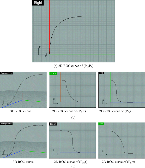
2. Despite the fact that an ROC curve of (
PD,
PF) is generated by varying
PF, actually both
PD and
PF are determined by the threshold τ and functions of τ where each pair of (
PD,
PF) is obtained by a single value of threshold τ. Unfortunately, a direct relationship between
PD and
PF via τ is hidden in the 2D ROC curve of (
PD,
PF). As a consequence, it may occur that two different detectors δ
1 and δ
2 may generate the same 2D ROC curves of (
PD,
PF) as shown in
Figure 3.5(a) but their 3D ROC curves along with the other two 2D ROC curves of (
PD,τ) and (
PF,τ) are in fact quite different as shown in
Figures 3.5(b), and
3.5(c).
The example illustrated in
Figure 3.5 demonstrates that the traditional ROC analysis is ineffective in capturing the impact and effect of different threshold values on
PD and
PF individually. As will also be demonstrated in the experiments, the 2D ROC curves of (
PD,τ) and (
PF,τ) provide certain crucial information about how to choose a best possible threshold τ to compromise
PD and
PF, a task that the 2D ROC curve of (
PD,
PF) cannot really deliver.
3. The traditional 2D ROC analysis generally makes an assumption that the noise is Gaussian so that a closed form for the 2D ROC curve of (
PD,
PF) can be generated analytically in such a way that
PD can be expressed as a function of
PF without actually calculating the threshold τ. However, in many real-world applications the Gaussian assumption is usually not valid. In this case, no analytical form for an ROC curve of (
PD,
PF) can be derived. Accordingly, we need to consider the original detector structure in
(3.5) where the threshold τ is the key parameter that determines the detector performance. The 3D ROC curve provides an exit tool from this dilemma to represent detection performance in terms of the three parameters
PD,
PF, and τ where both
PD and
PF can be expressed as functions of τ as shown in
Figures 3.4(c) and
3.4(d).