4.3 Six Scenarios of Synthetic Images
Section 4.2 describes how to simulate subsample targets or mixed-sample targets according to their characteristics. In this section, we will discuss on how to simulate synthetic images with target panels inserted in accordance with certain desired properties.
4.3.1 Panel Simulations
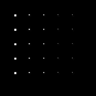
First, the real image scene with reflectance data shown in Figure 1.12(c) is used to simulate panels of interest where the reflectance spectra of five USGS ground-truth mineral spectra: alunite (A), buddingtonite (B), calcite (C), kaolinite (K), and muscovite (M) are used to simulate 25 panels of various sizes that are arranged in a ![]() matrix as shown in Figure 4.2.
matrix as shown in Figure 4.2.
Figure 4.2 25 simulated panels.

Each row of the five panels in Figure 4.2 is simulated by the same mineral signature and each column of five panels has the same size. Among 25 panels are five ![]() -pure pixel panels,
-pure pixel panels, ![]() for
for ![]() in the first column, five
in the first column, five ![]() -pure pixel panels,
-pure pixel panels, ![]() for
for ![]() in the second column, five
in the second column, five ![]() -mixed pixel panels,
-mixed pixel panels, ![]() for
for ![]() in the third column, five subpixel panels,
in the third column, five subpixel panels, ![]() for
for ![]() in the fourth column, and five subpixel panels,
in the fourth column, and five subpixel panels, ![]() for
for ![]() in the fifth column. The purpose of introducing five panels in the third column is to conduct a study and analysis on the five mineral signatures with different mixtures in a pixel. Table 4.1 tabulates the mixing details of mineral composition in the 20 panels in the third column, while subpixel panels in the fourth and fifth columns are simulated with their simulated abundance fractions tabulated in Table 4.2, where the background (BKG) is simulated by the sample mean of the real cuprite image scene in Figure 1.12(a).
in the fifth column. The purpose of introducing five panels in the third column is to conduct a study and analysis on the five mineral signatures with different mixtures in a pixel. Table 4.1 tabulates the mixing details of mineral composition in the 20 panels in the third column, while subpixel panels in the fourth and fifth columns are simulated with their simulated abundance fractions tabulated in Table 4.2, where the background (BKG) is simulated by the sample mean of the real cuprite image scene in Figure 1.12(a).
Table 4.1 Simulated 20 mixed panel pixels in the first column.
| Row 1 | ||
| Row 2 | ||
| Row 3 | ||
| Row 4 | ||
| Row 5 | ||
Table 4.2 Abundance fractions of subpixel panels in the fourth and fifth columns.
| Row | Fourth column | Fifth column |
| 1 | ||
| 2 | ||
| 3 | ||
| 4 | ||
| 5 |
According to Tables 4.1 and 4.2, the simulated synthetic image in Figure 4.2 has a total of 130 panel pixels present in the scene, 80 pure pixel panels in the first column, 20 pure pixel panels in the second column, 20 mixed panel pixels in the third column, five 50%-abundance subtarget panel pixels in the fourth column, and five 25%-abundance subpixel target panel pixels in the fifth column. These 130 pixel panels include a total of 26 spectrally distinct signatures (5 pure mineral signatures in the first and second columns, 20 mixed signatures in the third column 5 along with 1 BKG signature). Figure 4.3 graphically plots the abundance fractions of all these 130 panel pixels where (a-e) indicate the five mineral signatures, A, B,C,K, and M, used to simulate 26 panel pixels in each of five rows in Figure 4.2 respectively.
Figure 4.3 Graphical plots of abundance fractions of 130 panel pixels in Figure 4.2.

By virtue of the 25 simulated panels in Figure 4.2, two target insertions, TI and TE, can be designed to be used for experiments conducted in this book.
4.3.2 Three Scenarios for Target Implantation (TI)
Three interesting scenarios for TI, Scenario TI1, Scenario TI2, and Scenario TI3, presented in this section, are designed for applications in target extraction such as endmember extraction (see Part II) and target quantification. The 25 panels in Figure 4.2 are used as targets of interest and implanted in a synthetic image scene with size of ![]() pixel vectors in a way that the targets to be implanted replace their corresponding background pixels. Each of these three scenarios is described as follows.
pixel vectors in a way that the targets to be implanted replace their corresponding background pixels. Each of these three scenarios is described as follows.
4.3.2.1 Scenario TI1 (Clean Panels Implanted into Clean Background)
This scenario assumes that the image background is clean and simulated by only one BKG signature. The 25 clean panels simulated in Figure 4.2 are then implanted in the background by replacing their corresponding background pixels with the clean panel pixels. The resulting image is a synthetic image shown in Figure 4.4 with clean panels implanted in the clean background image scene.
Figure 4.4 Synthetic image simulated by Scenario TI1.

4.3.2.2 Scenario TI2 (Clean Panels Implanted into Noisy Background)
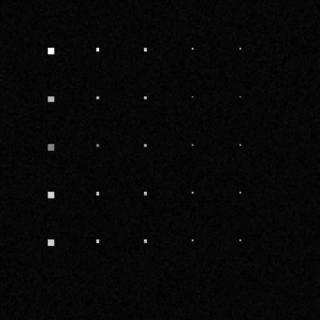
Practically, Scenario TI1 does not exist because of no noise present in the data. Scenario TI2 is more realistic when the noise-free background in Scenario TI1 is replaced with a noisy background image which is corrupted by an additive Gaussian noise to achieve a signal-to-noise ratio (SNR) = 20:1 defined as 50% signature (i.e., reflectance/radiance) divided by the standard deviation of the noise in Harsanyi and Chang (1994). Then clean targets are implanted into such simulated noisy background image. So, the resulting synthetic image has clean targets implanted in a noisy background as shown in Figure 4.5. This scenario simulates a case that true clean targets are indeed present in a noisy image background for target extraction.
Figure 4.5 Synthetic image simulated by Scenario TI2.

The synthetic image scene in this scenario is the same as the one in Scenario TI1 except that the image background is not clean, but rather corrupted by an additive Gaussian noise with SNR = 20:1.
4.3.2.3 Scenario TI3 (Gaussian Noise Added to Clean Panels Implanted into Clean Background)
Scenario TI3 is the same as Scenario TI1 except that a Gaussian noise is added to TI1 to achieve an SNR = 20:1. So, in this synthetic image, the clean targets and clean background image are both corrupted by an additive Gaussian noise with SNR = 20:1 as shown in Figure 4.6. It is also similar to Scenario TI2 but the implanted targets are now noise-corrupted compared to the clean targets implanted in Scenario TI2.
Figure 4.6 Synthetic image simulated by Scenario TI3.

This scenario simulates a case that the implanted targets are not original true targets and have been contaminated and corrupted by noise. As a consequence of noise corruption, all the pure pixels, mixed pixels, and subpixels are contaminated. So, technically, those panel pixels of 100% purity as endmembers are no longer pure. However, these implanted targets are still considered to be purest and closest to the original targets compared to other pixels present in the image scene. So, they can still be considered as targets of interest. This scenario is designed to test and evaluate how sensitive a target extraction algorithm can be when clean targets are corrupted by noise.
4.3.3 Three Scenarios for Target Embeddedness (TE)
In the previous sections, three scenarios for TI are simulated by inserting the 25 panels into the image scenes by removing background pixels to accommodate these 25 panels for target implantation. As an alternative, this section simulates another type of target insertion, called TE, which inserts the 25 panels into an image scene with a size of ![]() pixel vectors by adding the 25 panels directly to an image scene in such a way that the 25 panels are simply superimposed over their corresponding background pixels. In other words, unlike target implantation in Scenarios TI1, TI2, and TI3 which replaced background pixels with 25 implanted panel pixels, the following three scenarios embed 25 panel pixels by adding panel pixels to background pixels via superimposition. In this case, a pixel which contains an embedded panel pixel also contains a background pixel and thus, its abundance is the sum of abundance of the embedded panel pixel and background pixel. The three counterparts of Scenarios TI1, TI2, and TI3 can also be simulated as TE1, TE2, and TE3, respectively. The design of TE serves different applications such as signal detection (see Chapter 2) and discrimination including subpixel target detection and discrimination, mixed pixel classification, and identification.
pixel vectors by adding the 25 panels directly to an image scene in such a way that the 25 panels are simply superimposed over their corresponding background pixels. In other words, unlike target implantation in Scenarios TI1, TI2, and TI3 which replaced background pixels with 25 implanted panel pixels, the following three scenarios embed 25 panel pixels by adding panel pixels to background pixels via superimposition. In this case, a pixel which contains an embedded panel pixel also contains a background pixel and thus, its abundance is the sum of abundance of the embedded panel pixel and background pixel. The three counterparts of Scenarios TI1, TI2, and TI3 can also be simulated as TE1, TE2, and TE3, respectively. The design of TE serves different applications such as signal detection (see Chapter 2) and discrimination including subpixel target detection and discrimination, mixed pixel classification, and identification.
4.3.3.1 Scenario TE1 (Clean Panels Embedded in Clean Background)
Scenario TE1 is the same as Scenario TI1 except that the targets implanted into the background are now embedded into the background as shown in Figure 4.7.
Figure 4.7 Synthetic image simulated by Scenario TE1.

More specifically, the targets are inserted into the background in such a manner that the targets are added to their corresponding background pixels without removing them similar to Scenario TI1. This scenario simulates an idealistic case for signal detection where two hypotheses represent background versus signal plus background, that is, H0: BKG versus H1: clean signal + BKG. As a result, there are no pure pixels in this particular scenario since pure pixels in the first and second columns are no longer pure due to its inclusion of background pixels. So, technically, there are no pure signatures or endmembers in the image scene, but there are 25 spectrally distinct panel signatures plus one BKG signature.
4.3.3.2 Scenario TE2 (Clean Panels Embedded in Noisy Background)
In analogy with TI2, Scenario TE2 simulates a practical signal detection problem where clean targets are embedded into a noisy background simulated by a background signature with an additive Gaussian noise to achieve an SNR = 20:1. In other words, instead of replacing background pixels with the clean targets as done in Scenario TI2, the targets are actually embedded into and superimposed over clean background pixels. So, in this case, the resulting synthetic image has clean targets embedded into a noisy background as shown in Figure 4.8.
Figure 4.8 Synthetic image simulated by Scenario TE2.

This scenario simulates a case for target detection where two hypotheses represent noisy background against signal plus noisy background, that is, H0: BKG + noise versus H1: clean signal + BKG + noise. It is tricky to simulate this scenario since the noisy background pixels are replaced by their corresponding clean background pixels, while SNR must be retained at the given level.
4.3.3.3 Scenario TE3 (Gaussian Noise Added to Clean Panels Embedded in Background)
Scenario TE3 is the same as Scenario TE1 except that a Gaussian noise is added to Scenario TE1 to achieve SNR = 20:1 as shown in Figure 4.9.
Figure 4.9 Synthetic image simulated by Scenario TE3.

It is also similar to Scenario TE2 with only difference that the embedded targets are noise corrupted compared to the clean targets embedded in Scenario TE2. More specifically, in Scenario TE3 the clean targets and clean background image are both corrupted by an additive Gaussian noise with SNR = 20:1. So, the 25 spectrally distinct panel signatures are corrupted by noise and BKG signature. This scenario simulates a case that two hypotheses represent noisy background against noisy signal with noisy background, i.e., H0: noisy BKG versus H1: noisy signal + noisy BKG.
Finally, several remarks on the above designed six synthetic images are noteworthy:
