1.7 Real Hyperspectral Images to be Used in this Book

Three real hyperspectral image data sets are frequently used in this book for experiments. Two are AVIRIS real image data sets, Cuprite in Nevada and Purdue's Indian Pine test site in Indiana. A third image data set is HYperspectral Digital Imagery Collection Experiment (HYDICE) image scene. Each of these three data sets is briefly described as follows.

1.7.1 AVIRIS Data

Two AVIRIS data sets presented in this section are Cuprite data and Purdue's data, which can be used for different purposes in applications. The Cuprite data set is generally used for endmember extraction and target detection, while the Purdue's data set is mainly used for land cover/land use classification.

1.7.1.1 Cuprite Data

One of the most widely used hyperspectral image scenes available in the public domain is Cuprite mining site, Nevada, as shown in Figure 1.11(a). It is an image scene of 20 m spatial resolution collected by 224 bands using 10 nm spectral resolution in the range of 0.4–2.5 μm. The center region shown in Figure 1.11(b), cropped from the image scene in Figure 1.10(a), has size of pixel vectors.

Figure 1.11 Cuprite image scene, (a) original Cuprite image scene; (b) the image cropped from the center region of the original scene in (a) (). (See the color version of this figure in Color Plates section).

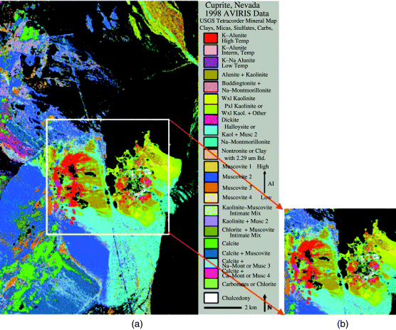
Since it is well understood mineralogically and has reliable ground truth, this scene has been studied extensively. Two data sets for this scene, reflectance and radiance data, are also available for study. There are five pure pixels in Figure 1.11(a, b) that can be identified to be corresponding to five different minerals, alunite (A), buddingtonite (B), calcite (C), kaolinite (K), and muscovite (M) labeled by A, B, C, K, and M, respectively, in Figure 1.12(b) with their corresponding reflectance and radiance spectra shown in Figure 1.12(c, d).

Figure 1.12 (a) Spectral band number 170 of the Cuprite AVIRIS image scene; (b) spatial positions of five pure pixels corresponding to minerals: alunite (A), buddingtonite (B), calcite (C), kaolinite (K), and muscovite (M); (c) reflectances of five minerals marked in (b) in wavelengths; (d) radiances of five minerals marked in (b) in bands; and (e) alteration mineral map available from USGS. (See the color version of this figure in Color Plates section).

These five pure pixels are carefully verified using laboratory spectra provided by the USGS (available from http://speclab.cr.usgs.gov) and selected by comparing their reflectance spectra in Figure 1.12(c) against the lab reflectance data in Figure 1.9. Figure 1.12(e) also shows an alteration map for some of the minerals, which is generalized from ground map provided by the USGS and obtained by Tricorder SW version 3.3. It should be noted that this radiometrically calibrated and atmospherically corrected data set available from http://aviris.jpl.nasa.gov is provided in reflectance units with 224 spectral channels where the data has been calibrated and atmospherically rectified using the ACORN software package. It is recommended that bands 1–3, 105–115, and 150–170 be removed prior to data processing due to their low water absorption and low SNR. As a result, a total of 189 bands are used for experiments as shown in Figure 1.11(c, d). The steps to produce spectra in Figure 1.12(c, d) can be described as follows:

It should be noted that the ground truth is not stored in a “file.” The locations of the five minerals are identified by comparing their reflectance spectra against their corresponding lab reflectances in the spectral library.

1.7.1.2 Purdue's Indiana Indian Pine Test Site

Another most widely used real AVIRIS image data set is Purdue's Indiana Indian Pine test site, which has 20 m spatial resolution and 10 nm spectral resolution in the range of 0.4–2.5 μm with size of pixel vectors taken from an area of mixed agriculture and forestry in Northwestern Indiana, USA. The data set is available on the web site http://cobweb.ecn.purdue.edu/~biehl/MultiSpec/documentation.html (both download link and ground truth are provided) and was recorded in June 1992 with 220 bands with water absorption bands, bands 104–108 and 150–162 removed and leaving only 202 bands. Figure 1.13(a) shows nine bands selected from the web site and a USGS quadrangle map of the test site provided in Figure 1.13(b).

Figure 1.13 AVIRIS image scene: Purdue Indiana Pine test site. (a) Nine bands selected from the Purdue Indiana Pine test site; (b) a USGS quadrangle map of the test site; (c) ground truth of Purdue Indiana Pine test site; and (d) ground truth of each of 17 classes. (See the color version of this figure in Color Plates section).

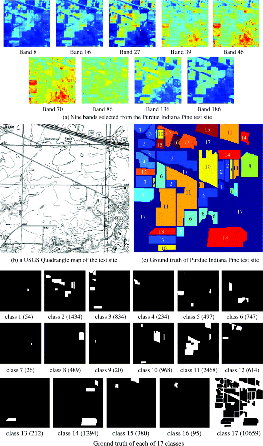
According to the ground truth provided in Figure 1.13(c) there are 17 classes in this image scene shown in Figure 1.13(d) including the background labeled by class 17, which has a wide variety of targets such as highways, railroad, houses/buildings, and vegetation that may not be of interest in agricultural applications but may be of great interest in other applications such as anomaly detection. The total number of data samples in the scene is . Table 1.2 lists labels of each of 17 classes where the numeral in parenthesis under each of 17 classes in Figure 1.13(d) is the number of data samples in that particular class.

Table 1.2 Labels of 17 classes.

Due to the early season of harvest when the data were collected, some cultivated land has very little canopy cover. For example, the corn area can be divided into three classes based on how much is left on the land, which are corn-no till, -min, and corn (class 2–4). The soybean area also can be divided into soybean-no till, -min, and -clean (class 10–12). The grass is mixed with four other materials, which are classified as grass/pasture, grass/trees, grass/pasture-mowed, and bldg-grass-green-drives (class 5, 6, 7, 15). Actually, it is believed that the grass is also mixed in the background. According to Figure 1.13(c, d) (Landgrebe, 2003), the GIS map in Figure 1.13(b) provides the information of “land use” classes instead of “land cover” classes. It means that not every pixel in the map is supposed to be classified into their belonging classes. Additionally, also based on the USGS quadrangle map in Figure 1.13(b), there are dual lane highways (U.S. 52 and 231) and a railroad crossed near the top. The other is Jackson highway, which is near to the middle of the scene. All of them are in the NW–SE direction. Figure 1.13(b) also indicates some houses or buildings by small rectangular dots (Landgrebe, 1998). With this information it is believed that there are at least four classes included in the background: railroad (iron), highway (concrete), houses/buildings (concrete, painted wood, or other materials), and vegetation (grass). The number of classes for such unlabeled areas is important for the unsupervised classification when the total number of classes in the scene is assumed to be unknown.

There are many reasons to select the Purdue Indiana Indian Pine test site for experiments. First of all, it is a well-known image scene available on web site and has been studied extensively. Another is that the pixels in this image scene are heavily mixed. Many algorithms or methods claiming to work well on classification are very likely to break down for this image scene. To the author' best knowledge, most work on this image scene reported in the literature has selected particular areas for study and also supervised based on the provided ground truth. Very little has been done in classification of the entire scene either supervisedly or unsupervisedly. Most interestingly, according to our detailed analysis on the scene, we have found that it is almost impossible to classify all the 17 classes in the image scene even though the complete knowledge of the ground truth provided in Figure 1.13(c, d) is used for classification. This is because pixels in the same class are mixed so badly that values among their spectral signatures measured by any spectral similarity measure vary in a relatively wide range in which pixels in the same class may be classified into different classes and pixels in different classes may be considered to belong to the same class.

From the ground truth provided in Table 1.2, it can be expected that the signatures of three subclasses of corn are close to each other, so are the four subclasses of grass and three subclasses of soybean. However, the relationships among other pairs are still not known. In order to know how much mixing is involved, the signature for each class is calculated by averaging all samples with the same label according to the ground-truth map in Figure 1.12(c). Then the SAM is used to measure how close one class is similar to the other. It has been shown in Liu (2005) that corn and soybean classes (2–4, 10–12) are similar, which account for 6552 pixels, 63% of 10,366 labeled pixels. Similarity also appears in two sets of classes: class 1, 7, 8 and class 6, 9, 13. Surprisingly, the four classes of grass (5, 6, 7, 15), which account for 1650 pixels, are not similar to each other. Additionally, using SAM to measure spectral similarity among 16 classes, it is found that classes 5, 14, 16 seem to be the three most distinct classes and can be classified very easily. It is reasonable and makes sense because class 5 contains chlorophyll, class 14 is wood, and class 16 comprises man-made objects.

With our tremendous experience of working on this image scene, excluding two classes (class 17 that is considered to be the background and class 9 that is considered to be too small) it is found that the spectral signatures of the pixels in the six classes (class 2, class 3, class 4, class 7, class 9, and class 11) are very close in terms of SAM or SID (spectral information divergence in Chang (2003a)). Similarly, the pixels in the three classes (class 8, class 10, and class 15) also have very similar spectral signatures. Hence distinguishing one from another is very difficult. The pixels in the three classes (class 13, class 5, and class 14) have less similar signatures but still present some difficulty with classification. The most dissimilar classes are class 1, class 6, and class 12 that are considered to be easy to classify. By taking into account all the things considered above, we can expect that the classification of this image scene is a great challenge to any hyperspectral imaging algorithm.

1.7.2 HYDICE Data

The HYDICE image scene shown in Figure 1.14(a) has a size of pixel vectors along with its ground truth provided in Figure 1.14(b) where the center and boundary pixels of objects are highlighted by red and yellow, respectively. The upper part contains fabric panels with size 3, 2, and 1 m² from the first column to the third column. Since the spatial resolution of the data is 1.56 m², the panels in the third column are considered as subpixel objects. The lower part contains different vehicles with sizes of (the first four vehicles in the first column) and (the bottom vehicle in the first column) and three objects in the second column (the first two have size of 2 pixels and the bottom one has size of 3 pixels, respectively). In this particular scene, there are three types of targets with different sizes, small-size targets (panels of three different sizes, 3, 2, and 1 m²), and large-size targets (vehicles of two different sizes, and and three objects of 2-pixel and 3-pixel sizes) that can be used to validate and test anomaly detection performance.

Figure 1.14 HYDICE vehicle scene. (a) Image scene; (b) ground-truth map; (c) five vehicles; and (d) ground truth of (c). (See the color version of this figure in Color Plates section).

Figure 1.14(c) shows an enlarged HYDICE scene from the same flight for visual assessment. It has a size of pixel vectors with 10 nm spectral resolution and 1.56 m spatial resolution where five vehicles lined up vertically to park along the tree line in the field where the red (R) pixel vectors (shown as dark pixels) in Figure 1.14(d) show the center pixel of the vehicles, while the yellow (Y) pixels (shown as bright pixels) are vehicle pixels mixed with background pixels.

A third enlarged HYDICE image scene shown in Figure 1.15(a) is also cropped from the upper part of the image scene in Figure 1.14(a, b) marked by a square.

Figure 1.15 (a) A HYDICE panel scene that contains 15 panels; (b) ground-truth map of spatial locations of the 15 panels. (See the color version of this figure in Color Plates section).

It has a size of pixel vectors with 15 panels in the scene. This particular image scene has been well studied in Chang (2003a). Within the scene there is a large grass field background, a forest on the left edge, and a barely visible road running on the right edge of the scene. Low signal/high noise bands: bands 1–3 and bands 202–210; and water vapor absorption bands: bands 101–112 and bands 137–153 were removed. The spatial resolution is 1.56 m, and spectral resolution is 10 nm. There are 15 panels located in the center of the grass field and are arranged in a matrix as shown in Figure 1.15(b), which provides the ground-truth map of Figure 1.15(a). Each element in this matrix is a square panel and denoted by p_ij with row indexed by i = 1, ..., 5 and column indexed by j = 1, 2, 3. For each row i = 1, ..., 5, the three panels were painted by the same material but have three different sizes. For each column j = 1, 2, 3, the five panels have the same size but were painted by five different materials. It should be noted that the panels in rows 2 and 3 are made by the same material with different paints, so did the panels in rows 4 and 5. Nevertheless, they were still considered as different materials. The sizes of the panels in the first, second, and third columns are 3 m × 3 m, 2 m × 2 m, and 1 m × 1 m, respectively. So, the 15 panels have 5 different materials and 3 different sizes. Figure 1.15(b) shows the precise spatial locations of these 15 panels where red pixels (R pixels, i.e., dark pixels) are the panel center pixels and the pixels in yellow (Y pixels, i.e., bright pixels) are panel pixels mixed with background. The 1.56 m spatial resolution of the image scene suggests that the panels in the second and third columns, denoted by p₁₂, p₁₃, p₂₂, p₂₃, p₃₂, p₃₃, p₄₂, p₄₃, p₅₂, p₅₃ in Figure 1.15(b) are one pixel in size. Additionally, except the panel in the first row and first column, denoted by p₁₁ which also has a size of one pixel, all other panels located in the first column are two-pixel panels, which are the panels in the second row with two pixels lined up vertically, denoted by p₂₁₁ and p₂₂₁; the panel in the third row with two pixels lined up horizontally, denoted by p₃₁₁ and p₃₁₂; the panel in the fourth row with two pixels also lined up horizontally, denoted by p₄₁₁ and p₄₁₂; and the panel in the fifth row with two pixels lined up vertically, denoted by p₅₁₁ and p₅₂₁. Since the size of the panels in the third column is 1 m × 1 m, they cannot be seen visually from Figure 1.15(a) due to its size being smaller than the 1.56 m pixel resolution.

Figure 1.16 plots the five panel spectral signatures obtained from Figure 1.15(b), where the ith panel signature, denoted by p_i was generated by averaging the red panel center pixels in row i. These panel signatures will be used to represent target knowledge of the panels in each row.

Figure 1.16 Spectra of p₁, p₂, p₃, p₄, and p₅.

According to visual inspection and ground truth in Figure 1.15(a, b) there are also four background signatures shown in Figure 1.17, which can be identified and marked by interferer, grass, tree, and road. These four signatures along with five panel signatures in Figure 1.16 can be used to form a 9-signature matrix for a linear mixing model to perform supervised linear spectral mixture analysis.

Figure 1.17 Areas identified by ground truth and marked by three background signatures, grass, tree, road plus an interferer. (See the color version of this figure in Color Plates section).