30.6 Experiments for Concealed Target Detection

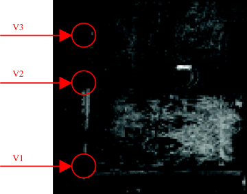
Two HYDICE datasets to be used in the experiments were two different image scenes taken in Maryland in August 1995 using 210 bands with spectral coverage 0.4–2.5 μm of resolution 10 nm and GSD approximately 0.78 m. Figure 30.6 shows an image scene with size of pixel vectors. Three vehicles of the same type are parked underneath the trees on the left edge and aligned vertically and circled by V1, V2, and V3 from bottom to top. Except V1, which is partially revealed, the other two vehicles V2 and V3 are completely concealed.

Figure 30.6 A HYDICE image scene.

In this experiment, BBOPC used a two-layer pyramid to reduce the image size and generated seven bands (band numbers: 16, 41, 53, 57, 63, 83, and 96) with for band ratio transformation, which resulted in band-ratioed images obtained by (30.7). It was then followed by ATGP where 12 target signatures were detected and generated and each target signature was classified in an individual image. It should be noted that many of the targets detected were background signatures such as grass, trees, or unknown interferers. Figure 30.7(a) only shows that three vehicles V1, V2, and V3 in Figure 30.6 were effectively detected and classified by CADCA. Since CADCA is an abundance estimation-based classifier, the resulting images were gray-scaled. In order to segment the detected and classified targets from the background, we used a Winner-Take-All (WTA) rule to threshold the gray-scaled image in Figure 30.7(a) and produced its thresholded image in Figure 30.7(b) where only concealed vehicles were shown in the image. The WTA rule used here was based on the maximum of abundance fractions resident within a pixel. It calculated the abundance fractions of 12 target signatures present in a pixel vector estimated by CADCA and assigned the pixel the target whose value yielded the maximal abundance. As a result of this WTA assignment, a gray-scaled image in Figure 30.7(a) was converted to a binary image in Figure 30.7(b) with one assigned to the target and zero otherwise.

Figure 30.7 Detected concealed targets: (a) gray-scaled image; (b) thresholded image.

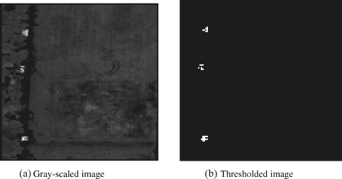
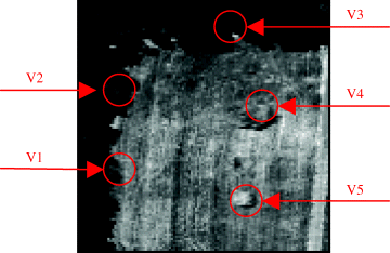
Figure 30.8 shows another HYDICE image scene of size pixel vectors and has a large grass field with tree lines running along the left edge and three vehicles are parked underneath trees where there are two vehicles, circled by V1 (bottom one) and V2 (upper one) along with the left tree line and a third circled by V3 hidden under the top tree line. In addition to these three vehicles, two different material-made objects, circled by O1 (bottom one) and O2 (upper one), are located near the center to the left. Covered under O1 and O2 are two vehicles, indicated V4 and V5, respectively. Except V2, all other four vehicles, V1, V3, V4, and V5, belong to the same type of vehicles. As shown in Figure 30.8, all five vehicles are completely concealed. Only visible targets in the figure are O1 and O2. Apparently, from Figure 30.8, there are no clues about these vehicles and their corresponding locations.

Figure 30.8 Another HYDICE image scene.

Similarly, Figure 30.9(a) shows gray-scaled images resulting from applying CADCA to Figure 30.8 where seven bands (band numbers: 16, 53, 56, 60, 63, 82, and 96) were also selected by BBOPC using a two-layer pyramid and threshold for band ratio transformation. The resulting band-ratioed images were used for ATGP to detect and generate 24 target signatures for classification. Like Figure 30.7, most of the detected targets in Figure 30.8 were uninteresting or unwanted background signatures. As shown in Figure 30.9, V1 was detected in Figure 30.9(a) while V2 and V3 were detected in Figure 30.10(c). Further, V4 and V5 were also detected in Figure 30.9(b) and (d), respectively (see bright spots within the two objects, O1 and O2).

Figure 30.9 Detected concealed targets.

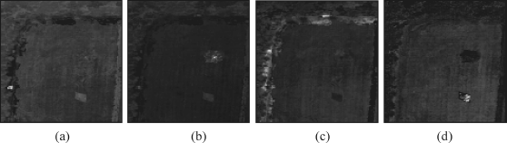
Figure 30.10 Detected concealed targets.

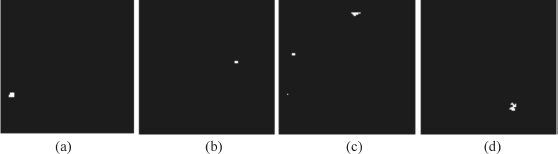
Figure 30.10 shows thresholded binary images of Figure 30.10(a–d) obtained by WTA where V1, {V2,V3}, V4, and V5 were detected in Figure 30.10(a), 30.10(c), 30.10(b), and 30.11(d), respectively.

As noted, V2 and V3 are different vehicles but were classified as the same type of vehicles because their spectra were very close. Furthermore, despite the fact that V4 and V5 are of the same type of vehicles, they were detected and classified in two different images because the two objects O1 and O2 used to cover these two vehicles are made by different materials. These results were interesting. Unlike V1, V2 and V3 which are shaded by trees, V4 and V5 are hidden underneath O1 and O2.