32.6 Real MR Brain Image Experiments

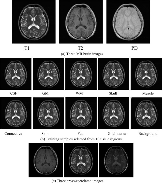
The real MR images used for experiments were obtained in the TaiChung Veterans General Hospital (TCVGH) to further validate the utility of the proposed LSMA-based intrapixel techniques in real images in calculating partial volumes of brain tissues. The MR images shown in Figure 32.23(a) were obtained from one normal volunteer by a whole body 1.5-T MR system (Sonata, Siemens, Erlangen, Germany). The routine brain MR protocol consisted of axial spin echo T1 weighted images (TR/TE = 400/9 ms), proton density image (TR/TE = 4000/10 ms), and T2 weighted images (TR/TE = 4000/91 ms). Other imaging parameters included for this experiment were slice thickness = 6 mm, matrix = 256 × 256, field of view (FOV) = 24 cm, and number of excitations (NEX) = 2. These images are shown in Figure 32.23(a). Training sample sets for 10 classes were selected according to their anatomical structures shown in Figure 32.23(b).

Figure 32.23 Three real MR images in (a) along with training samples in (b).

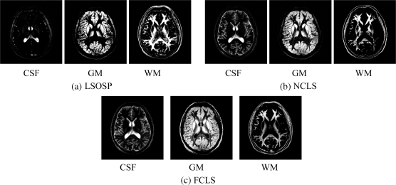
By visual inspection of Figures 32.23–32.26, the PVE results produced by all the techniques separated the three major substances clearly in general. However, there were also some supposedly WM substances showing in GM-generated images by all the techniques. Moreover, similar to the synthetic brain image experiment, OSP and LSOSP produced similar estimated abundances and so did NCLS and FCLS. Another observation is that the skull showed up in the WM images generated by all the techniques. This suggested that using a skull stripping as a preprocessing to remove the skull prior to classification may actually improve PVE results.

Figure 32.24 Classification results of the original real MR images produced by (a) LSOSP, (b) NCLS, and (c) FCLS.

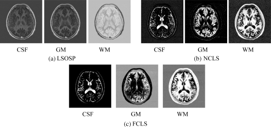
Figure 32.25 Classification results of the three main brain tissues with BEP-expanded six bands (T1, T2, PD, and cross-correlation BEP) produced by (a) OSP, (b) LSOSP, (c) NCLS, and (d) FCLS techniques with five substances (CSF, GM, WM, skull, and background).

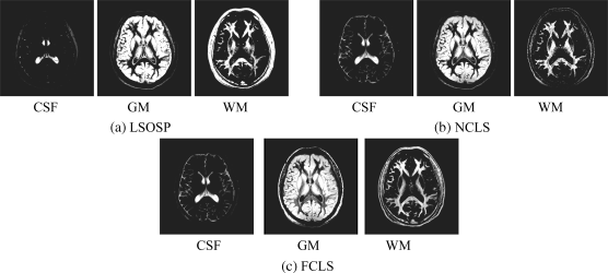
Figure 32.26 Classification results of three main brain tissues with BEP expanded nine bands (T1, T2, PD, cross-correlation BEP, and auto-correlation BEP) produced by (a) LSOSP, (b) NCLS, and (c) FCLS with five substances (CSF, GM, WM, skull, and background).

With this image dataset including three original images in Figure 32.23(a) and three additional BEP-generated images in Figure 32.23(c), the same experiments conducted for the synthetic images in Section 32.4 were repeated where the training samples from GM, WM, CSF, and skull were selected by an experienced radiologist, as shown in Figure 32.27.

Figure 32.27 Tissues training sample regions for CSF, GM, WM, and skull for the real brain MR images.

In addition to the four tissues in Figure 32.27, a fifth tissue signature used as a background signature was obtained by taking the average over other unwanted tissue signatures plus the actual background of MR images to form a five-signature matrix M to be used for LSMA to unmix the three main brain tissues of interest, CSF, GM, and WM as their PVEs. Figures 32.28(a)–(c), 32.28(d)–(f), and 32.28(g)–(i) show the PVE results of CSF, GM, and WM using three non-kernel-based LSMA methods (LSOSP, NCLS, and FCLS), three K-LSMA methods (K-LSOSP, K-NCLS, and K-FCLS), and three K-BEP-LSMA methods (K-BEP-LSOSP, K-BEP-NCLS, and K-BEP-FCLS), respectively.

Figure 32.28 Classification results of three main brain tissues of real brain MR image produced by (a) LSOSP, (b) NCLS, (c) FCLS, (d) K-LSOSP, (e) K-NCLS, (f) K-FCLS, (g) K-BEP-LSOSP, (h) K-BEP-NCLS, and (i) K-BEP-FCLS with five substances (CSF, GM, WM, skull, and background).

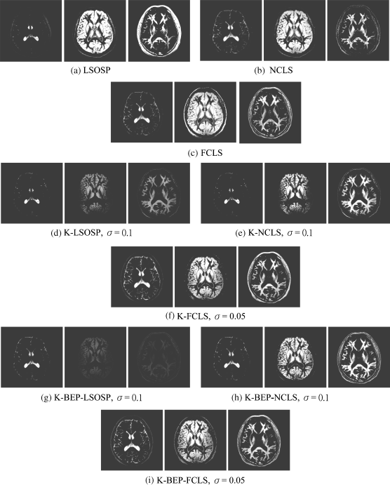
The parameter σ used in the RBF kernels by K-LSMA was emperically chosen by σ = 0.1 for K-LSOSP, K-BEP-LSOSP, K-NCLS, and K-BEP-NCLS and σ = 0.05 for K-FCLS and K-BEP-FCLS. According to the results shown in Figure 32.28, NCLS demonstrated the best classification in terms of their unmixed PVEs among all LSMA methods. In particular, CSF and GM were classified correctly with little false positive classification as shown in Figure 32.28(b), (e), and (h) when NCLS, K-NCLS, and K-BEP-NCLS were used. On the other hand, the worst performance was LSOSP-based methods. As shown in Figures 32.28(a), (d), and (g), WM was classified with significant false positives from skull and muscle when LSOSP, K-LSOSP, and K-BEP-LSOSP were used. Generally speaking, K-LSMA improved the false positive classification rate. In particular, the false classification of the skull and muscle tissues into WM for LSOSP shown in Figure 32.28(a) was significantly reduced as shown in Figure 32.28(d). Similar to synthetic image experiments, K-BEP-LSMA had very little improvement on the false positive classification.