10.7 Synthetic Image Experiments

Once again the synthetic images described in Chapter 4 were used for experiments to evaluate the performance of the proposed REEAs. Scenarios TI1 and TE1 were not included in the experiments because there is no randomness caused by noise, in which case REEAs do not work in this scenario due to the fact that they are designed as random algorithms. Three component transform techniques, PCA, MNF and ICA, were used to perform DR to reduce the original data space to a reduced data space with data dimensionality determined by VD.

10.7.1 RPPI

The experiments of RPPI were implemented by 500 skewers on two data sets, a reduced data cube by DR and the original data without DR where the data dimensionality to be retained after DR was n_VD = 5 estimated by the NWHFC method with P_F = 10⁻⁴. Figures 10.1(a) and (b) and 10.2(a) and (b) show the results for TI2 and TI3 produced by PPI and RPPI, respectively, where pixel vectors in Figures 10.1(a) and 10.2(a) marked by open circles were extracted by PPI with PPI counts greater than zero and all pixel vectors in Figures 10.1(b) and 10.2(b) were those in the intersection of all runs by RPPI. As shown in Figures 10.1 and 10.2, the number of pixels extracted by RPPI as endmembers was significantly reduced with only less than 10 falsely alarmed endmembers in Figures 10.1(a) and 10.2(a) compared to a very large number of pixels extracted by PPI in Figures 10.1(a) and 10.2(a) as endmembers with hundreds of falsely alarmed pixels.

Figure 10.1 Endmembers extracted by PPI and RPPI in scenario TI2.

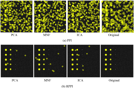
Figure 10.2 Endmembers extracted by PPI and RPPI in scenario TI3.

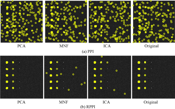
Similarly, Figures 10.3(a) and (b) and 10.4(a) and (b) show the results for TE2 and TE3 produced by the PPI and RPPI, respectively, where pixel vectors in Figures 10.3(a) and 10.4(a) marked by open circles were extracted by the PPI with PPI counts greater than zero and all pixel vectors in Figures 10.3(b) and 10.4(b) were those in the intersection of all runs by RPPI. Since there are no pure pixels present as endmembers in TE2 and TE3, PPI and RPPI made attempt to extract pixels that represent purest signatures. As expected, more falsely alarmed endmember pixels than those in Figures 10.1(b) and 10.2(b) were extracted as shown in Figures 10.3(b) and 10.4(b). Interestingly, in the case of TE3 RPPI missed all the pure pixels in row 3 if it is implemented directly on the original data without DR. Besides, if PCA was used for DR, RPPI missed all the 16 purest panel pixels in the first column of row but it did extract panel pixels in the second column. This is mainly due to the fact that the calcite signature is very similar and close to the sample mean used to simulate the image background. As a result, the calcite was considered as a variant of the background signature and thus was not extracted as purest signature in Figure 10.4(b) by RPPI.

Figure 10.3 Endmembers extracted by PPI and RPPI in scenario TE2.

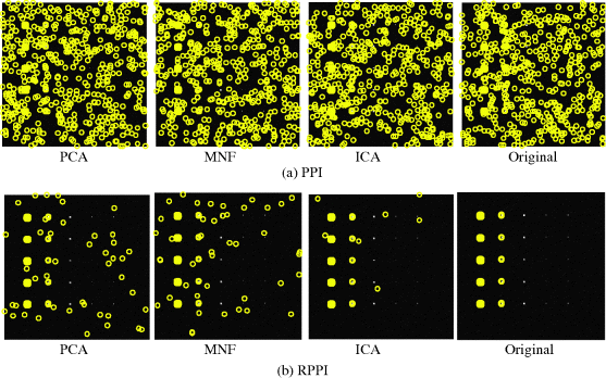
Figure 10.4 Endmembers extracted by PPI and RPPI in scenario TE3.

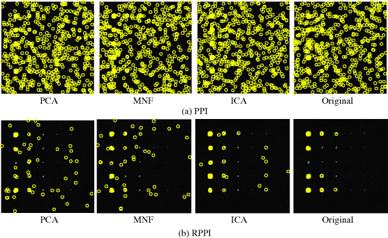
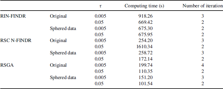
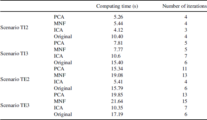
Table 10.1 tabulates the number of iterations and the computing time in seconds for RPPI to converge. As expected, except TE3 RPPI operating on the original data space without DR generally required the maximal computing time, while RPPI required the least amount of computing time if the ICA was used for DR.

Table 10.1 Computing time and the number of iterations of RPPI running in different data sets.

10.7.2 Various Random Versions of IN-FINDR

A random version of N-FINDR, RN-FINDR, is quite different from RPPI presented in Section 10.6.1. First is the prior knowledge. RN-FINDR needs to know the number of endmembers, p, to be generated, which is not required for PPI but is traded off for two must-be-known parameters, the number of skewers, K, and the threshold t. Second is data to be processed. PPI generally requires DR as a preprocessing to reduce data dimensionality to compact information as well as reduce computational complexity. On the other hand, RN-FINDR does not perform DR. Instead, it spheres the data to remove the statistics of the first and second order to enhance and improve endmember extraction. In order to illustrate RN-FINDR for the performance evaluation, the experiments conducted in this section were particularly designed to address two main issues: (1) inconsistency caused by the use of two randomly generated sets of initial conditions, and (2) two different data sets to be used for processing, the original data and sphered data. Three random versions of N-FINDR were used for a comparative study, RIN-FINDR, RSC N-FINDR, and RSGA, all of which were implemented without DR. The number of endmembers required to be generated by RN-FINDR for all the four synthetic image-based scenarios, TI2, TI3, TE2, and TE3, was determined by VD, which was 2n_VD = 10 for all the algorithms.

10.7.2.1 Scenario TI2

Figures 10.5–10.10 show the results of IN-FINDR, SC N-FINDR, and SGA along with their corresponding random counterparts, RIN-FINDR, RSC N-FINDR, and RSGA for TI2. There were two sets of endmembers generated in Figures 10.5, 10.7, and 10.9 by operating IN-FINDR, SC N-FNDR, and SGA on the original data and sphered data to illustrate inconsistent final results from the use of two randomly generated initial conditions. In contrast, Figures 10.6, 10.8, and 10.10, respectively, show the consistent final results of operating the RIN-FINDR, RSC N-FINDR, and RSGA on the original data and sphered data using two thresholds τ = 0.05 and 0.005. It should be noted that since SC N-FINDR and SGA are SQ-EAAs, the endmembers were labeled by numbers to indicate the orders in which they were generated. However, there were no numbers associated with IN-FINDR-generated endmembers because these endmembers were generated iteratively at the same time.

Figure 10.5 Results of IN-FINDR with two different runs for TI2.

Figure 10.6 Results of RIN-FINDR with two different thresholds for TI2.

Figure 10.7 Results of SC N-FINDR with two different runs for TI2.

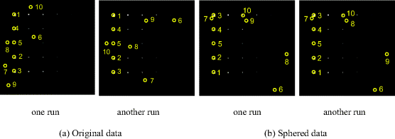
Figure 10.8 Results of RSC N-FINDR with two different thresholds for TI2.

Figure 10.9 Results of SGA with two different runs for TI2.

Figure 10.10 Results of RSGA with two different thresholds for TI2.

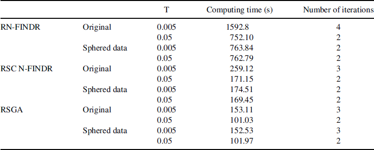
Comparing the results in above figures, it is interesting to note that it only required the first five pixels for SC N-FINDR and the first six pixels for SGA to extract all the five mineral signatures as endmembers where the first pixels extracted by SGA were always background pixels. Nevertheless, with p set by 2n_VD = 10 all the algorithms successfully extracted pixels that specify all the five mineral signatures as endmembers. Table 10.2 tabulates the computing time and the number of iterations required for a random algorithm to complete its search where RSGA required the least amount of computing time which was only one-seventh of time required by RIN-FINDR. However, it should be noted that the computing time needed by REEAs was heavily determined by the number of iterations required to complete the endmember search.

Table 10.2 Computing time and number of iterations for RN-FINDR, RSC N-FINDR, and RSGA.

10.7.2.2 Scenario TI3

Despite that the 100 pure panel pixels in TI3 have been Gaussian noise-corrupted, these pure panel pixels no longer represent pure signatures but they are still those with purest signatures. Figures 10.11–10.16 show that for p = 2n_VD = 10, IN-FINDR, SC N-FINDR, and SGA along with their random versions, RIN-FINDR, RSC N-FINDR, and RSGA were all able to extract panel pixels which represented most purest signatures corresponding to the five distinct minerals. However, the threshold value, τ, used by the random versions of N-FINDR should have a greater threshold tolerance to accommodate the added Gaussian noise such as τ = 0.05. If the threshold value was set too small, e.g., τ = 0.005 used for TI2, random versions of N-FINDR would miss one mineral signature, M in row 5 in Figures 10.12, 10.14, and 10.16.

Figure 10.11 Results of IN-FINDR with two different runs.

Figure 10.12 Results of RIN-FINDR with two different thresholds.

Figure 10.13 Results of SC N-FINDR with two different runs.

Figure 10.14 Results of RSC N-FINDR with two different thresholds.

Figure 10.15 Results of SGA with two different runs.

Figure 10.16 Results of RSGA with two different thresholds.

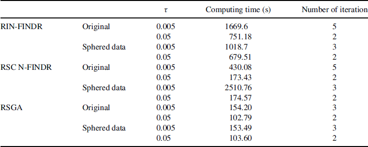
Table 10.3 tabulates the computing time and the number of iterations required for a random algorithm to complete its search, where RSGA required the least amount of computing time. The computing time documented in the table was essentially determined by the number of iterations required to complete the endmember search.

Table 10.3 Computing time and number of iterations for RIN-FINDR, RSC N-FINDR, and RSGA.

10.7.2.3 TE2

Following the same treatment carried out for TI2, experiments were also conducted for TE2. The only difference is that the pure panel pixels are superimposed over the background pixels in which case no pure signatures are present in TE scenarios. Nevertheless, the purest pixels in TE2 were still the same as the pure panel pixels in TI2. Figures 10.17–10.22 show that all algorithms were able to extract panel pixels corresponding to the five distinct mineral signatures. Specifically, the RIN-FINDR and RSC N-FINDR extracted the same identical five panel pixels that corresponded to the five distinct pure mineral signatures.

Figure 10.17 Results of IN-FINDR with two different runs.

Figure 10.18 Results of RIN-FINDR with two different thresholds.

Figure 10.19 Results of SC N-FINDR with two different runs.

Figure 10.20 Results of RSC N-FINDR with two different thresholds.

Figure 10.21 Results of SGA with two different runs.

Figure 10.22 Results of RSGA with two different thresholds.

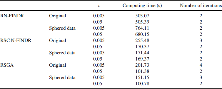
Table 10.4 tabulates the computing time and the number of iterations required for a random algorithm to complete its search where once again RSGA required the least amount of computing time.

Table 10.4 Computing time and number of iterations for RN-FINDR, RSC N-FINDR, and RSGA.

10.7.2.4 TE3 Scenario

TE3 is an additive Gaussian noise-corrupted scenario of TE2. Figures 10.23–10.28 show the results of IN-FINDR, SC N-FINDR, and SGA along with their random counterparts. Analogous to TI3, it was expected that a larger threshold value, τ = 0.05, was also required for random versions of N-FINDR to combat the added Gaussian noise so that panel pixels with the purest signatures that represented the five distinct mineral signatures could be extracted as shown in Figures 10.24, 10.26, and 10.28.

Figure 10.23 Results of IN-FINDR with two different runs.

Figure 10.24 Results of RIN-FINDR with two different thresholds.

Figure 10.25 Results of SC N-FINDR with two different runs.

Figure 10.26 Results of RSC N-FINDR with two different thresholds.

Figure 10.27 Results of SGA with two different runs.

Figure 10.28 Results of RSGA with two different thresholds.

Table 10.5 tabulates the computing time and the number of iterations required for a random algorithm to complete its search where once again RSGA required the least amount of computing time.

Table 10.5 Computing time and number of iterations for RIN-FINDR, RSC N-FINDR, and RSGA.