Chapter 8
Selecting Secondary Features
When you need to create features that are somewhat outside the mainstream, you may need to reach deeper into SolidWorks. SolidWorks has lots of functionality that lies out of the public eye that may be just what you are looking for in certain situations. You probably will not use the tools you find in this chapter every day, but knowing about them may mean the difference between having the capability and not having it.
Creating Curve Features
Curves in SolidWorks are often used to help define sweeps and lofts, as well as other features. Curves differ from sketches in that curves are defined using sketches or a dialog box, and you cannot manipulate them directly or dimension them in the same way that you can sketches. Functions that you are accustomed to using with sketches often do not work on curves.
These curve features are covered in this chapter:
- Projected Curve
- Helix and Spiral
- Curve Through XYZ Points
- Curve Through Reference Points
- Composite Curve
- Imported Curve
Several features that carry the curve name are actually sketch-based features:
- 3D Sketch
- Equation-Driven Curve
- Intersection Curve
- Face Curve
Split Line is another feature that can create edges on faces that can be used like curve features. Split Lines can function as curves in some situations, so this section discusses the Split Line along with the rest of the curve and other curve-like features.
Of these, the Projected and Helix curves are by far the most frequently used, but the others may be important from time to time. Curve functions do not receive much attention from SolidWorks. Updates to curve features are few, and in some cases the functions are buggy. The usefulness of curve features is limited in the software, but in some cases there is no other good way to achieve the same result.
You can find all the curve functions on the Curves toolbar or by choosing Insert ➢ Curve from the menu. Curve features, in general, have several limitations; some of them are serious. You often have to be prepared with workaround techniques when using them.
Manipulating Curves
Curves cannot be mirrored, moved, patterned, or manipulated in any way. (A workaround for this may be to use Convert Entities to create a sketch from the curve, or to create a surface using the curve, and pattern or mirror the surface, using the edge of the surface in place of the curve feature.)
Working with Helix Curve Features
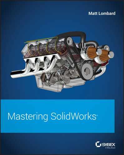
![]() The Helix curve types are all created from a sketch circle. The circle represents the starting plane, center, and diameter of the helix. Figure 8.1 shows the PropertyManagers of the Constant Pitch and Variable Pitch helix types.
The Helix curve types are all created from a sketch circle. The circle represents the starting plane, center, and diameter of the helix. Figure 8.1 shows the PropertyManagers of the Constant Pitch and Variable Pitch helix types.

FIGURE 8.1 The Helix/Spiral PropertyManager
You can create all the helical curve types by specifying some combination of total height, pitch, and the number of revolutions. The start angle depends on the relation of the sketch plane to the origin. The start angle can be controlled outside of the PropertyManager through dimensions, design tables, equations, and so forth. The term pitch refers to the straight-line distance along the axis between the rings of the helix. Pitch for the spiral is different and is described later.
USING THE TAPER HELIX PANEL
The Taper Helix panel in the Helix PropertyManager enables you to specify a taper angle for the helix. The taper angle does not affect the pitch. If you need to affect both the taper and the pitch, you can use a Variable Pitch helix. Figure 8.2 shows how the taper angle relates to the resulting geometry.

FIGURE 8.2 The Taper Helix panel
USING THE VARIABLE PITCH HELIX
You can specify a Variable Pitch helix either in the chart or in the callouts that are shown in Figure 8.3. Both the pitch and the diameter are variable. The diameter number in the first row cannot be changed but is driven by the sketch. In the chart shown, the transition between 4 and 4.5 revolutions is where the pitch and diameter both change.
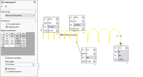
FIGURE 8.3 The Variable Pitch helix
When you double-click a helix feature, SolidWorks displays the dimensions on the screen, which you can then double-click and change. The dimensions displayed this way aren't as organized as when using the PropertyManager, but it may be more convenient.
ESTABLISHING A WORKFLOW
One workflow for all the Helix-type curves is as follows:
- Draw a circle or select an existing circle.
- Start the Helix command.
- Set the options.
- Click the green checkmark icon to accept the feature.
USING THE SPIRAL
A spiral is a flattened (planar) tapered helix. The pitch value on a spiral is the radial distance between revolutions of the curve. (See Figure 8.4.)

FIGURE 8.4 The Spiral option of the Helix feature
Creating Projected Curves
![]() There are two types of projected curves:
There are two types of projected curves:
- Sketch On Faces
- Sketch On Sketch
These names can be misleading if you do not already know what they mean. In both cases, the word sketch is used as a noun, not a verb, so you are not actively sketching on a surface; instead, you are creating a curve by projecting a sketch onto a face.
USING SKETCH ON FACES
With this option set, the projected curve is created by projecting a 2D sketch onto a face. The sketch is projected normal (perpendicular) to the sketch plane. The sketch can be an open loop or a closed loop, but it may not be multiple open or closed loops, nor can it be self-intersecting. Figure 8.5 shows an example of projecting a sketch onto a face to create a projected curve.

FIGURE 8.5 A projected curve using the Sketch On Faces option
USING SKETCH ON SKETCH
The easiest method to use for visualizing Sketch On Sketch projected curves is the Intersecting Surfaces method. In this method, you can see the curve being created at the intersection of two surfaces that are created by extruding each of the sketches. This method is shown in Figure 8.6.
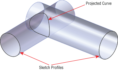
FIGURE 8.6 Using intersecting surfaces to visualize a Sketch On Sketch projected curve
Using the Curve Through XYZ Points Feature
![]() The Curve Through XYZ Points feature enables you to either type or import a text file with coordinates for points on a curve. The text file can be generated by any program that makes lists of numbers, including Excel. The curve reacts like a default spline, so the teeter-tottering effect may be noticeable, especially because you cannot set end conditions or tangency. To avoid this effect, it may be a good idea to overbuild the curve by a few points on each end or to have a higher density of points.
The Curve Through XYZ Points feature enables you to either type or import a text file with coordinates for points on a curve. The text file can be generated by any program that makes lists of numbers, including Excel. The curve reacts like a default spline, so the teeter-tottering effect may be noticeable, especially because you cannot set end conditions or tangency. To avoid this effect, it may be a good idea to overbuild the curve by a few points on each end or to have a higher density of points.
If you import a text file, the file can have an extension of either *.txt or *.sldcrv. The sample data file Chapter 8 - Curve File.sldcrv is in the download material. The data that it contains must be formatted as three columns of X-, Y-, and Z-coordinates using the document units (inch, mm, and so on), and the coordinates must be separated by a comma, space, or tab. Figure 8.7 shows both the Curve File dialog box displaying a table of the curve through X, Y, and Z points, and the *.sldcrv Notepad file. You can read the file from the Curve File dialog box by clicking the Browse button; but if you manually type the points, then you can also save the data out directly from the dialog box. Just like any type of sketch, this type of curve cannot intersect itself.
FIGURE 8.7 The Curve File dialog box showing a table of the curve through X, Y, and Z points, and a Notepad text file with the same information
Using the Curve Through Reference Points Feature
![]() The Curve Through Reference Points feature creates a curve entity from selected sketch points or vertices. The curve can be an open loop or a closed loop, but a closed loop requires that you select at least three points. You cannot set end conditions of the curve, so this feature works like a default spline in the same way as the XYZ curve.
The Curve Through Reference Points feature creates a curve entity from selected sketch points or vertices. The curve can be an open loop or a closed loop, but a closed loop requires that you select at least three points. You cannot set end conditions of the curve, so this feature works like a default spline in the same way as the XYZ curve.
The most common application of this feature is to create a wire from selected points along a wire path. Another common application is a simple two-point curve to close the opening of a surface feature such as Fill, Boundary, or Loft. One drawback in that regard is that the end tangency directions cannot be controlled on curve features. If a 3D sketch spline is used, end tangency direction is controlled easily through the use of spline handles and tangency to construction geometry. Curve Through Reference Points is largely unused, probably because 3D sketch splines are so much more powerful.
Putting Together a Composite Curve
![]() A composite curve joins multiple curves, edges, or sketches into a single curve entity. The spring shown in Figure 8.8 was created by using a composite curve to join a 3D sketch, Variable Pitch helix, and projected curve. You can also use model edges with a composite curve. The curve is shown on half of the part; the rest of the part is mirrored. Curves cannot be mirrored, but solid/surface geometry can.
A composite curve joins multiple curves, edges, or sketches into a single curve entity. The spring shown in Figure 8.8 was created by using a composite curve to join a 3D sketch, Variable Pitch helix, and projected curve. You can also use model edges with a composite curve. The curve is shown on half of the part; the rest of the part is mirrored. Curves cannot be mirrored, but solid/surface geometry can.
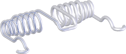
FIGURE 8.8 A part created from a composite curve
Composite curves overlap in functionality with the Selection Manager to some extent. In some ways, the composite curve is nicer because you can save a selection in case the creation of the feature that uses the Selection Manager fails. (If you can't create the feature, you can't save the selection.) On the other hand, composite curves don't function the same way as a selection of model edges for settings like tangency and curvature.
Using Split Lines
![]() Split lines are not exactly curves; they are just edges that split faces into multiple faces. Split lines are used for several purposes, but they are primarily intended to split faces so that draft can be added. They are also used for creating a broken-out face for a color break or to create an edge for a hold-line fillet, as discussed in Chapter 7, “Modeling with Primary Features.”
Split lines are not exactly curves; they are just edges that split faces into multiple faces. Split lines are used for several purposes, but they are primarily intended to split faces so that draft can be added. They are also used for creating a broken-out face for a color break or to create an edge for a hold-line fillet, as discussed in Chapter 7, “Modeling with Primary Features.”
There are some limitations to using split lines. First, they must split a face into at least two fully enclosed areas. You cannot have a split line with an open-loop sketch where the ends of the loop are on the face that is to be split; they must either hang off the face to be split or be coincident with the edges. If you think you need a split line from an open loop, try using a projected curve instead.
Using the Equation-Driven Curve
![]() An equation-driven curve is not really a curve feature; it is a sketch entity. It specifies a spline inside a 2D sketch with an actual equation. Even though this is a spline-based sketch entity, it can be controlled only through the equation and not by using spline controls. This feature is covered in more detail in Chapter 3, “Working with Sketches and Reference Geometry,” with other sketch entities.
An equation-driven curve is not really a curve feature; it is a sketch entity. It specifies a spline inside a 2D sketch with an actual equation. Even though this is a spline-based sketch entity, it can be controlled only through the equation and not by using spline controls. This feature is covered in more detail in Chapter 3, “Working with Sketches and Reference Geometry,” with other sketch entities.
Selecting a Specialty Feature
SolidWorks contains several specialty features that perform tasks that you will use less often than some of the standard features mentioned in Chapter 7, “Modeling with Primary Features.” Although you will not use these features as frequently as others, you should still be aware of them and what they do—you never know when you will need them.
These features include:
- Scale
- Dome
- Wrap
- Flex
- Deform
- Indent
Other types of less commonly used features fall into specialty categories such as sheet metal, multibodies, surfacing, plastics, and mold design. This includes features such as Freeform, Combine, Cavity, Scale, and several others. I placed the discussion about these features in chapters devoted to those specialized topics. The features discussed in this chapter are more general-use features.
Using Scale
![]() The Scale feature, found at Insert ➢ Feature ➢ Scale, is mainly used for preparing models of plastic parts to make mold cavity geometry; however, it can be used for any purpose on solid or surface geometry. Scale does not act by scaling up dimensions for individual sketches and features; rather, it scales the entire body at the point in the FeatureManager history at which it is applied. The Scale PropertyManager is shown in Figure 8.9.
The Scale feature, found at Insert ➢ Feature ➢ Scale, is mainly used for preparing models of plastic parts to make mold cavity geometry; however, it can be used for any purpose on solid or surface geometry. Scale does not act by scaling up dimensions for individual sketches and features; rather, it scales the entire body at the point in the FeatureManager history at which it is applied. The Scale PropertyManager is shown in Figure 8.9.

FIGURE 8.9 Applying the Scale feature
The Scale feature becomes available only when the part contains at least one solid or surface body. You can scale multiple bodies at once and select from one of three options for the Scale About setting or fixed reference: the part origin, the geometry centroid, or a custom coordinate system. Of these, it is generally preferable to select the part origin because you most often want the standard planes moving with respect to the rest of the part as little as possible. If you needed to scale about a specific point on the geometry, you would need to create a custom coordinate system at that point and use that as the reference.
The Scale Factor works like a multiplier, so if you want to double the length, you would enter the Scale Factor 2. This does not work like the Scale function in the Cavity feature, which is less commonly used. Scale within Cavity uses a scale factor that is shown as a percentage increase, so to double the linear dimensions of a part would require a scale factor of 100 percent. The Cavity feature is available only in the context of an assembly and has fallen out of favor with most mold designers.
Scale is also configurable, meaning that different configurations can use different scale factors. Configurations are covered in Chapter 11, “Working with Part Configurations.”
An interesting aspect of the Scale feature is that you can disable the Uniform Scaling option. This allows you to apply separate scale factors for the X, Y, and Z directions. In mold making, this can be used if you have a fiber-filled material and the mold requires differential shrink compensation based on the direction of plastic flow, and thus of fiber alignment (the part will shrink less in the direction of fiber alignment). But you could also use it to size any general part. Just remember that if you apply differential scale, circles may be distorted. To get around this, you may be able to reorder the features to apply the Scale feature before the circular features are added.
Because Scale is simply applied to the body rather than to features and sketches, it can be applied to imported parts as well as SolidWorks native parts. Sometimes, people use the Scale feature to compensate for improper imported units. For example, if a part was originally built in inches and translated in millimeters, you might want to scale the part by a factor of 25.4. You can also enter an expression in the Scale Factor box so that if the import units error went the other way, you could scale a part down by 1/25.4. The limitation to the Scale feature is that the SolidWorks modeling space for a single part is a box that’s approximately 500 to 700 meters centered about the origin. There appears to be some difference between sketching limits and 3D solid limits.
An implication of the Scale feature that is not stated outright is that it does not scale features, sketches, or dimensions. It is a history-based feature, so the size difference only applies after the Scale feature in the tree.
Using the Dome Feature
![]() The Dome feature in SolidWorks is generally applied to give some shape to flat faces or an area of a flat face. A great example of where a dome fits well is the cupped bottom of a plastic bottle or a slight arch on top of buttons for electronic devices. Domes can add or remove material.
The Dome feature in SolidWorks is generally applied to give some shape to flat faces or an area of a flat face. A great example of where a dome fits well is the cupped bottom of a plastic bottle or a slight arch on top of buttons for electronic devices. Domes can add or remove material.
Until SolidWorks 2010, another very similar feature existed, which was called Shape. You can no longer make Shape features, but you may run into one from time to time in old parts. If you find a Shape feature on an old part, it will continue to function unless any of its parent geometry changes. Shape features do not update in SolidWorks 2010 or later. SolidWorks recommends you re-create the geometry as another feature, possibly a Dome or Freeform feature. Included in the sample parts for Chapter 8 is a part called Chapter 8 Domes.sldprt; this part is shown in Figure 8.10. Opening this part will allow you to see the error that appears when you open a part with a Shape feature. The part also demonstrates several ways in which Dome features can be used.

FIGURE 8.10 Examples of various types of domes
The Dome feature has several attributes that either help it qualify for a given task or disqualify it. These attributes can help you decide if it will be useful in situations you encounter:
- The Dome feature can create multiple domes on multiple selected faces in a single feature, although it creates only a single dome for each face.
- Using the Elliptical Dome setting, Dome can create a feature that is tangent to the vertical.
- Dome can use a constraint sketch to limit its shape.
- Dome works on nonplanar faces.
- Dome cannot establish a tangent relationship to faces bordering the selected face.
- Dome cannot span multiple faces.
- Dome displays a temporary untrimmed four-sided patch that extends beyond the selected face when you use it on a non-four-sided face.
- Dome functions only on solids, not on surfaces.
The Dome feature has two notable settings: Elliptical Dome and Continuous Dome.
The Elliptical Dome is available only on flat faces where the boundary is either a complete circle or an ellipse. The cross section of the dome is elliptical and does not account for draft, which means that it is always tangent to the perpendicular from the selected flat face.
Continuous Dome is a setting for any noncircular or elliptical face, including polygons and closed-loop splines. The setting results in a single unbroken face. If you deselect the Continuous Dome setting, it functions like the Elliptical Dome setting. Figure 8.10 shows the most useful settings for the Dome feature.
The workflow for the Dome feature is as follows:
- Select an area to be domed, or use a split line to create an area to be domed on an existing face.
- Initiate the Dome feature, set a height, tell it to add or remove material, and set the other settings including the constraint sketch.
- Accept the feature with the green checkmark icon.
Using the Wrap Feature
![]() The Wrap feature enables you to wrap 2D sketches around analytical or complex faces. Trying to wrap around 360 degrees can cause some difficulties, so you might try that sort of thing in two steps, either with two wraps or a combination of features.
The Wrap feature enables you to wrap 2D sketches around analytical or complex faces. Trying to wrap around 360 degrees can cause some difficulties, so you might try that sort of thing in two steps, either with two wraps or a combination of features.
The Wrap feature works by flattening the face, relating the sketch to the flat pattern of the face, and then mapping the face boundaries and sketching back onto the 3D face. It is not a simple projection; it actually does wrap the sketch onto curved faces. Figure 8.11 shows the Wrap PropertyManager interface along with a Wrap onto a cylinder and a Wrap onto a complex shape. The complex wrap is available in the download materials for this chapter (see Complex Wrap.sldprt).
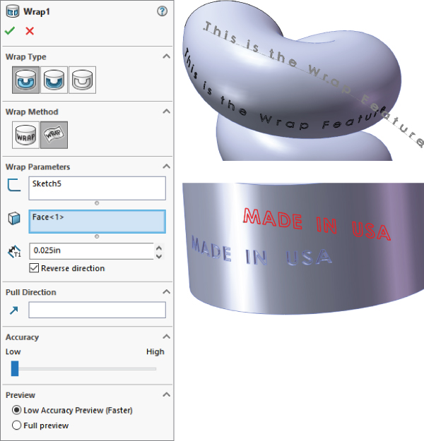
FIGURE 8.11 The Wrap PropertyManager interface
The Wrap feature has three main options:
- Emboss
- Deboss
- Scribe
Wrap can be placed on analytical (cylindrical, conical, and the like) or complex spline surfaces (lofts, sweeps, etc.).
USING SCRIBE
Scribe is the simplest of the options to explain, and understanding it can help you understand the other options. Scribe creates a split line–like an edge on the face.
Several requirements must be met in order to make a wrap feature work:
- The face must be a cylindrical or conical face.
- The loop must be a closed-loop or nested-closed-loop 2D sketch.
- The sketch must be on a plane that is either tangent to or parallel to another plane that is tangent to the face.
- Wrap supports wrapping onto multiple faces.
- The wrap should not be self-intersecting when it wraps around the part. (Self-intersection will not cause the feature to fail, but on the other types, Emboss and Deboss, it may produce unexpected results.)
Scribes can be created on solid or surface faces. Scribed surfaces are frequently thickened to create a boss or a cut. Figure 8.12 shows a scribed wrap.

FIGURE 8.12 The Wrap feature options
USING EMBOSS
The Wrap Emboss option works much like the scribe, but it adds material inside the closed-loop sketch, at the thickness that you specify in the Emboss PropertyManager. Embossing can be done only on solid geometry. If the feature self-intersects, then the intersecting area is simply not embossed and is left at the level of the original face. One result is that creating a full wraparound feature, such as the geometry for a barrel cam, requires a secondary feature. This is because the Wrap feature always leaves a gap, regardless of whether the sketch to be wrapped is under or over the diameter-multiplied-by-pi length.
When you use the Emboss option, you can set up the direction of pull and assign draft so that the feature can be injection molded. This limits the size of the emboss so that it must not wrap more than 180 degrees around the part.
USING DEBOSS
Deboss is just like emboss, except that it removes material instead of adding it. Figure 8.12 demonstrates all these options. The part shown in the images is available in the download material under the filename Chapter 8 Wrap.sldprt. For each of the demonstrated cases, the original flat sketch is shown to give you some idea of how the sketch relates to the finished geometry.
Keep in mind that this feature is not like the projected sketch. A projected sketch is projected normal from the sketch plane. A sketch that is 1-inch long when flat will measure 1 inch when wrapped along the curvature of the surface, and it will measure less than 1 inch linearly from end to end.
The embossed cam employed a workaround with a Revolve feature to close the gap that is always created when wrapping all the way around a part.
The example with the debossed text employs a direction of pull and draft so that the geometry can be molded. Sample models are available in the download material for Chapter 8 for Deboss, Emboss, and Scribe.
Using the Flex Feature
![]() The Flex feature is different from most of the other features in SolidWorks. Most of them create new geometry, but Flex (and Deform, which follows) takes existing geometry and changes its shape. Flex can affect the entire part or just a portion of it. Flex works on both solid and surface bodies, as well as imported and native geometry as shown in Figure 8.13.
The Flex feature is different from most of the other features in SolidWorks. Most of them create new geometry, but Flex (and Deform, which follows) takes existing geometry and changes its shape. Flex can affect the entire part or just a portion of it. Flex works on both solid and surface bodies, as well as imported and native geometry as shown in Figure 8.13.
![Flex dialog box displaying flex input having text box labeled Split1[2], twisting for selected radio button, and other details for Trim Plane 1, 2, Triad, Flex Options, with illustration of flex feature output on the right.](http://images-20200215.ebookreading.net/2/1/1/9781119300571/9781119300571__mastering-solidworks__9781119300571__images__c08f013.jpg)
FIGURE 8.13 The Flex feature creating a twist
Flex has four main options and many settings. The four main options are as follows:
- Bending: This option establishes two trim planes to denote the ends of the bent area and specifies an angle or radius for the bend.
- Twisting: This option establishes two trim planes to limit the area of the twist and enters the number of degrees through which to twist.
- Tapering: This option establishes two trim planes to limit the area of the taper. The body is larger toward one end and smaller toward the other end.
- Stretching: This option establishes two trim planes to limit the area to be stretched. You can stretch the entire body by moving the trim planes outside of the body.
The part shown in the figure can be found in the download material under the filename Chapter 8 Flex.sldprt.
In some cases, the Triad and trim planes are slightly disoriented. The best thing to do in situations like this is to simply reorient the Triad using the angle numbers in the Triad panel of the PropertyManager. This is also a solution if the planes are turned in such a way that the axis of bending is not oriented to the bend that the part requires.
The Flex feature is very conscious of separate bodies. In some cases this can be helpful, but in default situations when there is only one body in the part, it can be annoying. Remember to select the body to be affected in the very first selection box at the top of the PropertyManager.
You can place the trim planes by selecting a model vertex, by dragging the arrow on the plane, or by typing in a number. Be careful when dragging the plane arrows because dragging the border of the plane drags the flex value for the feature. (Dragging the plane in a bending operation is like changing the angle or radius for the bend.)
Using the Triad can be very tricky. Moving the Triad in the Bending option moves the axis of the bend, so it determines whether the bend compresses or stretches the material. The position of the Triad also determines which side of the bent body moves or stays stationary, or if both sides move. Placing the Triad directly on a trim plane causes the material outside the bend on that side of the trim plane to remain stationary.
I highly recommend looking at the models provided with this chapter to examine the various functions of the Flex feature more carefully. The model uses configurations, which are covered in Chapter 11, “Working with Part Configurations.”
Applying the Deform Feature
![]() Like the Flex feature, the Deform feature changes the shape of the entire model without regard to parametrics, features, history, or dimensions. Some software packages call this technique global shape modeling. Also like Flex, Deform works on surface bodies as well as solids. Deform can also handle imported geometry as well as SolidWorks native parts. Model complexity is not an issue unless the part runs into itself during deformation.
Like the Flex feature, the Deform feature changes the shape of the entire model without regard to parametrics, features, history, or dimensions. Some software packages call this technique global shape modeling. Also like Flex, Deform works on surface bodies as well as solids. Deform can also handle imported geometry as well as SolidWorks native parts. Model complexity is not an issue unless the part runs into itself during deformation.
The Deform feature is another feature type that you may not use to actually design anything, but you may use to show a model in a deformed state.
Deform has three types:
- Point: This type deforms a portion of the model by pushing a point and the geometry around it.
- Curve To Curve: The most precise and useful deform type. This type selects an existing edge and forces the edge to match a curve.
- Surface Push: This type of deform, while conceptually a very interesting function, is nearly unusable in practice. The part is deformed into a shape vaguely resembling an intermediate shape between the existing state of the part and a “tool” body.
Figure 8.14 shows the PropertyManager interface for the Deform feature. The interface is different for each of the three main types, and it changes depending on selections within the individual types. The interface shown is for the Curve To Curve type because I believe this to be the most useful type.
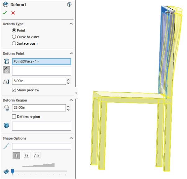
FIGURE 8.14 Using Deform to shape the chair back
LOOKING AT POINT DEFORM
The Point deform option enables you to push a point on the model, and the model deforms as if it were rubber. The key to using this feature is to ensure that the Deform Region option is unselected. Aside from that, you just have to use trial and error when applying the Point deform option. The depth, diameter, and shape of the deformation are not very precise. Also, you cannot specify the precise location for the point to be deformed. Again, this is best used for “looks-like” models, not production data.
LOOKING AT CURVE TO CURVE DEFORM
Because the Curve To Curve deform uses curve, sketch, or edge data, it is a more precise method than the other deform types. The main concept here is to transform a curve on the original model to a new curve, thereby deforming the body to achieve the new geometry.
The model shown in Figure 8.15 has been created using the Curve To Curve deform. The part starts as a simple sweep (sweep an arc along an arc), and then a split line is created to limit the deform to a specific area of the model. The model is in the downloaded files under the filename Chapter 8 Deform Curve to Curve.sldprt.

FIGURE 8.15 Using the Curve To Curve deform option
LOOKING AT SURFACE PUSH DEFORM
I don't go into much detail on the Surface Push deform type because it's not one of the more useful functions in SolidWorks. In order to use it, you must have the body of the part that you are modeling and a tool body that you will use to shape the part that you are modeling. The finished shape doesn't fit the tool body directly, but looks about halfway between the model and the tool body, blended together in an abstract sort of way. It looks like the dent that would result from an object being thrown very hard at a car fender, in that neither the thrown part nor the fender is immediately recognizable from the result.
Using the Indent Feature
![]() Indent uses the same ingredients as the Surface Push, but it produces a result that is more useful. For example, if you are building a plastic housing around a small electric motor, the Indent feature shapes the housing and creates a gap between the housing and the motor. Figure 8.16 shows the PropertyManager interface for the Indent feature, as well as what the indent looks like before and after using the feature.
Indent uses the same ingredients as the Surface Push, but it produces a result that is more useful. For example, if you are building a plastic housing around a small electric motor, the Indent feature shapes the housing and creates a gap between the housing and the motor. Figure 8.16 shows the PropertyManager interface for the Indent feature, as well as what the indent looks like before and after using the feature.
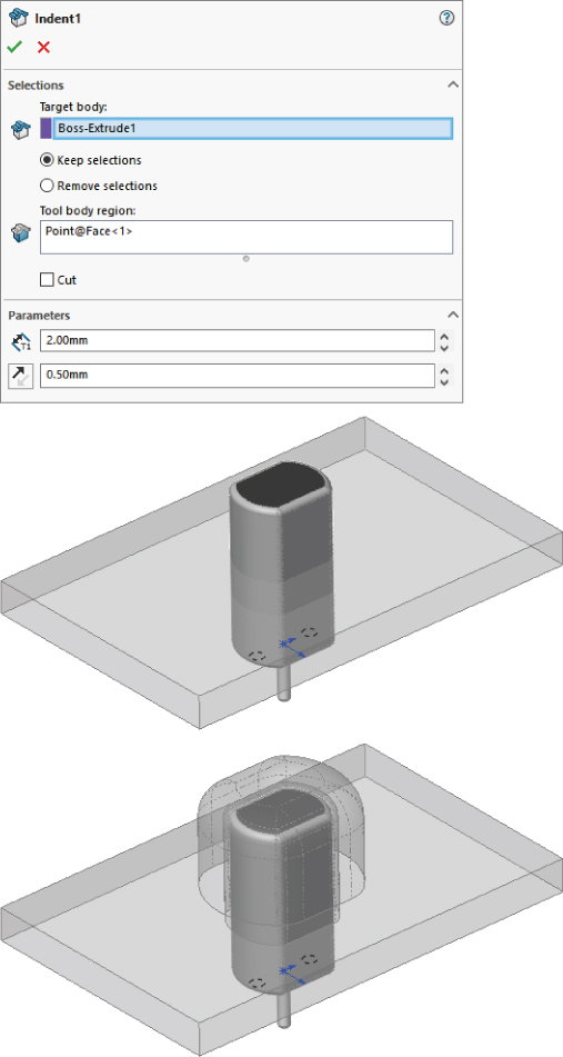
FIGURE 8.16 Using the Indent feature
In this case, the small motor is placed where it needs to be, but there is a wall in the way. Indent is used to create an indentation in the wall by using the same wall thickness and placing a gap of 0.010 inches around the motor. The motor is brought into the wall part using the Insert ➢ Part command. This is a multibody technique. Multibodies are examined in detail in Chapter 31, “Modeling Multibodies.”
It is possible to use Indent in mold applications; however, most mold designers will prefer to use the shrink percentage that you can get with the Scale/Cavity/Boolean operations rather than the discreet offset that Indent provides.
Using Intersect
![]() Intersect combines the functionality of general solids Boolean operations, Trim Surface, Knit Surface, Split, Replace Face, and Cut With Surface. The tool does not appear to have any exclusive functionality, but it reduces the work to complete some tasks that used to take many steps with a combination of different tools. It is useful for determining the volume of “open” cavities. For example, the part file shown in Figure 8.17 is a multibody with solids and surfaces. The small part in the center is a knob. The big block around it is a mold block, currently a single piece. The four cylinders are surfaces representing alignment pins, and the cylinder in the center is an ejector sleeve. The Top plane goes through the center and represents the parting line of the mold. You can find this part file in the download material for Chapter 8 under the filename
Intersect combines the functionality of general solids Boolean operations, Trim Surface, Knit Surface, Split, Replace Face, and Cut With Surface. The tool does not appear to have any exclusive functionality, but it reduces the work to complete some tasks that used to take many steps with a combination of different tools. It is useful for determining the volume of “open” cavities. For example, the part file shown in Figure 8.17 is a multibody with solids and surfaces. The small part in the center is a knob. The big block around it is a mold block, currently a single piece. The four cylinders are surfaces representing alignment pins, and the cylinder in the center is an ejector sleeve. The Top plane goes through the center and represents the parting line of the mold. You can find this part file in the download material for Chapter 8 under the filename Chapter 8 - Intersect Example.sldprt.
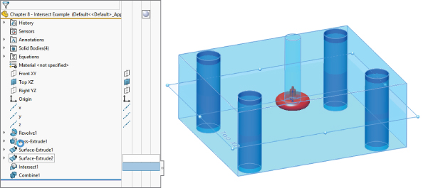
FIGURE 8.17 Creating a mold from representative solids and surfaces using Intersect: starting point
The first step is to select all the entities involved. This is much like the Mutual Trim feature. In the Selections panel of the Intersect PropertyManager, select every solid, surface, and plane that will take part in the operation.
You have the option to cap open surfaces while doing this, but this example does not require it. If one of the holes was a blind hole, but the surface body was open inside the solid, that situation would require a capped surface.
In this example, the only thing about the feature that is not very elegant is that the Merge result is not selective. Perhaps you can think of it as being the split function that is not selective. Notice that the final feature in the tree is a Combine. This was necessary because the original part was split into pieces. You may argue that the original part should be consumed—in which case, I wouldn't have allowed the pieces to remain—but this kind of decision should be up to the individual user, not the programmer.
The Consume Surfaces option simply removes any surface bodies used in the operation.
Tutorial: Creating a Wire-Formed Part
Follow these steps to create a wire-formed part:
- Open a new part using an inch-based template.
- Open a sketch on the Right (or Side) plane, and sketch a circle that is centered on the origin with a diameter of 1.500 inches.
- Create a Helix, Constant Pitch, Pitch, and Revolution, where Pitch = .250 inches, Revolutions = 5.15, and Start Angle = 0. The Helix command is found at Insert ➢ Curve ➢ Helix/Spiral.
- Create a sketch on the Front plane, as shown in Figure 8.18. Pay careful attention when adding the construction line, as shown. This line is used in the next step to reference the end of the arc.

FIGURE 8.18 The results up to step 4
- Open a sketch on the Right plane, and use the information from Figure 8.19 to add the correct relations and dimensions. Be aware that the two sketches shown are on different sketch planes, which makes it difficult to depict in 2D. You can also open the part from the download materials for reference.
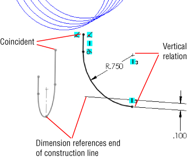
FIGURE 8.19 The sketch for step 5
- Exit the sketch and create a projected curve. The Projected Curve function is found at Insert ➢ Curve ➢ Projected Curve. Use the Sketch On Sketch option.
- Open a 3D sketch. You can access a 3D sketch from the Insert menu. Select the helix and click Convert Entities on the Sketch toolbar. Then select the projected curve, and click Convert Entities again. You now have two sections of a 3D sketch that are not connected in space.
- Draw a two-point spline to join the ends of the 3D sketch entities that are closest to one another. Assign tangent relations to the ends to make the transition smooth. Figure 8.20 illustrates what the model should look like at this point.
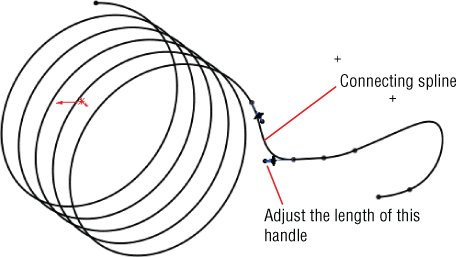
FIGURE 8.20 The results up to step 8
- Open a sketch on the Right plane, and draw an arc that is centered on the origin and coincident with the end of the 3D sketch helix. The 185-degree angle is created by activating the Dimension tool and clicking first the center of the arc and then the two endpoints of the arc. Now place the dimension. This type of dimensioning allows you to get an angle dimension without dimensioning to angled lines. Exit the sketch.
- Create a composite curve (Insert ➢ Curve ➢ Composite) consisting of the 3D sketch and the new 2D sketch.
- Create a new plane using the Normal To Curve option, selecting one end of the composite curve.
- On the new plane, draw a circle that is centered on the end of the curve with a diameter of 0.120 inches. You need to create a Pierce relation between the center of the circle and the composite curve.
- Create a Sweep feature using the circle as the profile and the composite curve as the path. To create the sweep, you must first exit the sketch.
- Hide any curves that still display.
- Choose Insert ➢ Cut ➢ With Surface. From the flyout FeatureManager, select the Right plane. Make sure the arrow is pointing to the side of the plane with the least amount of material. Click OK to accept the cut. The finished part is shown in Figure 8.21.
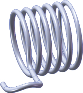
FIGURE 8.21 The finished part
The Bottom Line
SolidWorks has a wide range of features beyond the basic extrudes and revolves. You saw the depth of the standard features in Chapter 7 “Modeling with Primary Features”; now in Chapter 8, you have seen the breadth of some of the less-used, but still useful operations. You won't use each of these secondary features every day, but it is nice to know that if you need to show a model in a flexed in-use state, you at least don't have to directly model the deformed part manually. The need to custom-design springs in the design of small mechanisms is quite common. Having the ability to create such designs is a valuable skill.
- Master It Use a Helix and a 3D sketch to create a sweep path for a spring with elongated ends for use in a light mechanism.
Packaging and fixturing are additional types of design and modeling that are important for an engineer to master. Create a cavity such that the file named Chapter 8 Bottle.sldprt can nest into it.
- Master It Use the Indent feature to create the cavity in a thin sheet of material.
Text often has to go on irregular surfaces. Work through this example to gain some experience putting it there.
- Master It In the downloadable file
Chapter 8 Tutorial Bracket Casting.sldprt, some text is wrapped onto one of the cylindrical bosses. Put a model number on the second boss using the same process.