Note 17. FFT: Decimation-in-Time Algorithms

Consider the discrete Fourier transform for an N-point sequence

17.1

where

For even N, the DFT summation can be split into two separate summations—one for the even-indexed samples of x[n] and one for the odd-indexed samples.

17.2

Each of the summations in the final line of Eq. (17.2) is in the form of an (N/2)-point DFT. The signal flow graph (SFG) corresponding to the final line of Eq. (17.2) is shown in Figure 17.1 for the specific case of N = 8. In a circuit analysis context, SFGs often include curved lines, and the direction of signal flow is almost always indicated by an arrow. In a DSP context, it is conventional to use only straight edges, with signals flowing from left to right through the edges, unless indicated otherwise by the presence of an arrowhead. Each node represents a signal formed by the sum of all the inbound edges incident to the node.

Figure 17.1. Signal flow graph depicting operations defined by the final line of Eq. (17.2)

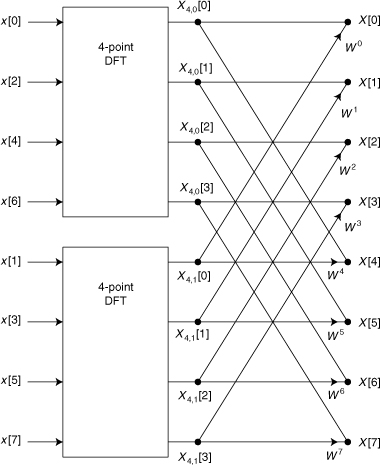
The node for X[0] in the upper right-hand corner of the figure has two incident edges. The lower edge, coming from node X_4,1[0], has a weight of W⁰, as indicated by the annotation near the arrowhead. The upper edge, coming from node X_4,0[0], has no weight indicated. This configuration of the node and the two incident edges indicates that

X[0] = X_4,0[0] + W⁰ X_4,1[0]

The complete set of equations represented by Figure 17.1 is

X[0] = X_4,0[0] + W⁰ X_4,1[0]

X[1] = X_4,0[1] + W¹ X_4,1[1]

X[2] = X_4,0[2] + W² X_4,1[2]

X[3] = X_4,0[3] + W³ X_4,1[3]

X[4] = X_4,0[0] + W⁴ X_4,1[4]

X[5] = X_4,0[1] + W⁵ X_4,1[5]

X[6] = X_4,0[2] + W⁶ X_4,1[6]

X[7] = X_4,0[3] + W⁷ X_4,1[7]

where the X_4,0[m] are the output of the upper, or “even,” 4-point DFT, and the X_4,1[m] are the outputs of the lower, or “odd,” 4-point DFT.

The weighting factors, W^k, have been called twiddle factors since the earliest days of digital signal processing. If N/2 is even, then the summations in Eq. (17.2) can each be split again. If N = 2^L, the summations at each stage can be split until the original transform is expressed as a combination of N 1-point DFTs. A 1-point transform is trivial:

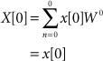
After L = log₂ N stages of splitting, all of the computational burden has been moved out of the summations and into the operations needed to combine 1-point transforms into 2-point transforms, 2-point transforms into 4-point transforms, and so on. The SFG for N = 8 and L = 3 is shown in Figure 17.2. Pairs of input points from x[n] are combined to form the eight values X_{2, k}[m] for k = 0, 1, 2, 3 and m = 0, 1. One complex multiply-add operation is required for each of the eight values.

Figure 17.2. Signal flow graph for 8-point decimation-in-time FFT with permuted inputs and naturally ordered outputs

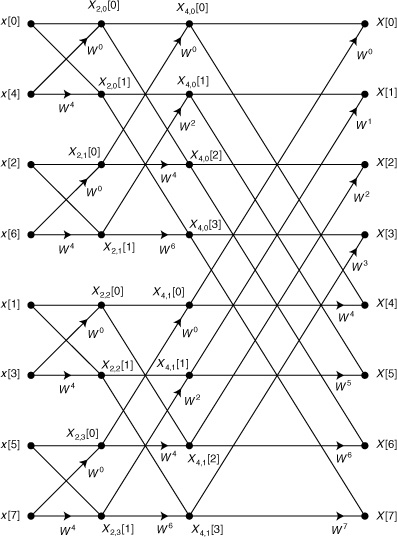
Figure 17.3. Signal flow graph for 8-point decimation-in-time FFT with naturally ordered inputs and permuted outputs

At the second stage, pairs of X_{2, k}[m] values are combined to form the eight values X_{4, k}[m] for k = 0, 1 and m = 0, 1, 2, 3. One complex multiply-add operation is required for computing each of the eight combinations.

Finally, pairs of X_{4, k}[m] values are combined to form the eight values X[m] for m = 0, 1, . . ., 7. In general, computing an N-point transform using this approach entails log₂ N stages of combining with N complex multiply-add operations per stage for a total computational burden of only N log₂ N complex multiply-add operations.

The output values, X[m], as shown in Figure 17.2, appear in “natural’’ order from X[0] through X[7]. The input values, x[n], appear in the permuted order x[0], x[4], x[2], x[6], x[1], x[5], x[3], x[7]. This order is called bit-reversed order because the index for the kth input value can be obtained by representing k with log₂ N bits and reversing the order of these bits. For example, when k = 3 = (011)₂, the corresponding bit-reversed index is (110)₂ = 6. Thus, the input x[6] appears in position 3 of the input sequence. The values x[0] and x[7] remain in their original positions because (000) and (111) are the same backward or forward. FFT algorithms of the type represented by Figure 17.2 are called decimation-in-time, permuted input-natural output (DIT-PINO) FFTs. It is possible to rearrange the nodes in Figure 17.2 without disturbing the connections between the nodes to obtain the SFG shown in Figure 17.3, where now the inputs are in natural order and the outputs are in bit-reversed order. This SFG represents a decimation-in-time, natural input-permuted output (DIT-NIPO) FFT.

17.1. Implementation Consideratons

For SFGs of FFTs that are drawn in “standard” form, the the edges connecting adjacent columns of nodes in can be grouped into patterns that are called butterflies because of their shape. Figure 17.4 shows the SFG of Figure 17.2, with one butterfly in each stage highlighted in bold. Figure 17.5 defines some convenient terminology we can use in this series of notes whenever butterflies and the operations that they represent are discussed.

Figure 17.4. Bold edges depict the butterfly structures embedded in the SFG for an FFT.

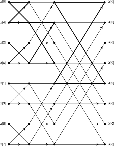
Figure 17.5. Butterfly terminology

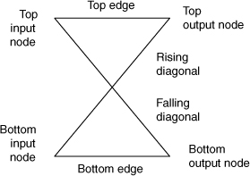
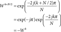
Let’s take a closer look at the butterflies in Figure 17.4 to uncover the patterns that are essential to software mechanization of the underlying mathematical operations. The first butterfly in stage 2 of the SFG of Figure 17.2 has X_2,0[0] and X_2,1[0] as its input nodes and X_4,0[0] and X_4,0[2] as its output nodes. The rising diagonal is multiplied by W⁰ and the bottom edge is multiplied by W⁴. The top edge and falling diagonal each have unity gain. Notice that for every butterfly in the SFG, when the rising diagonal is multiplied by W^k, the bottom edge is multiplied by W^k+N/2. Invoking the definition of W^k, it is easy to show that W^k+N/2= –W^k:

Thus, each butterfly can be implemented using a single complex multiplication and two complex additions. The bottom input node is multiplied by W^k to produce an interim result that is added to the top input node to obtain the top output node. The interim result is subtracted from the top input node to obtain the bottom output node. In an efficient implementation, all of the input nodes for a given stage are stored in a single array. Once the array location holding the bottom input node is used for computing the interim result, it is no longer needed and can be overwritten with the value computed for the butterfly’s bottom output node. The interim result can then be added to the array location holding the top input node to produce the top output node. The following fragment of C code summarizes this approach for butterfly implementation.

temp = array[bot_node_idx] * twiddle;
array[bot_node_idx]
       = aray[top_node_idx] - temp;
array[top_node] += temp;

The four butterflies in stage 1 of Figure 17.2 can all be computed in sequence using the single multiplier W⁰. There are two viable approaches for doing the stage-2 computations. The first approach computes the butterflies in order from top to bottom, generating (or perhaps recalling from storage) the multipliers W⁰, W², W⁰, and W² in sequence as they are needed. The second approach generates W⁰ only once, using it for each butterfly where it is needed before moving on to generate W². The first approach involves either extra trigonometry or storage for the multipliers. The second approach requires only slight additional complexity in the addressing scheme used to access locations in the node array.