Note 13. Discrete Fourier Transform
The discrete Fourier transform (DFT) is perhaps the single most important mathematical tool in all of DSP. Unlike many other Fourier analysis techniques that can be applied only to signals that are expressed in the form of mathematical functions, the DFT can be implemented in practical systems to analyze sampled real-world signals numerically. The DFT also plays a role in certain types of filter design as well as in the efficient implementation of filter banks, transmultiplexers, and demodulators for multi-frequency communication signals such as orthogonal frequency division multiplexing (OFDM).
Direct computation of an N-point DFT involves a number of arithmetic operations that is proportional to N2. There are many different algorithms that exploit periodicity, symmetry, and phase relationships in the sine and cosine functions to compute the DFT using significantly fewer arithmetic operations. These algorithms are collectively referred to as the fast Fourier transform (FFT). The most commonly used FFT algorithms require a number of arithmetic operations that is proportional to N log2N. The existence of these computationally efficient FFT algorithms makes real-time DFT analysis a viable choice for many DSP applications. This note deals with exploiting fundamental DFT behaviors and properties that are independent of the specific FFT mechanization that is ultimately selected.
The inverse DFT, or IDFT, is sometimes called the synthesis DFT because it can be used to synthesize a time-domain signal from a frequency-domain specification. Similarly, the forward DFT is sometimes called the analysis DFT because it can be used to analyze the frequency content of a time-domain signal.
Math Box 13.1. Discrete Fourier Transform
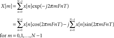
For a signal represented by an N-point sequence of samples, x[n], for n = 0, 1, . . ., N – 1, having a sample interval of T, the discrete Fourier transform (DFT) can be used to compute an estimate of the signal’s spectral content at the N discrete frequencies of 0, F, 2F, . . ., (N – 1)F, where F = (NT)–1. The DFT is defined by
MB 13.1
Inverse DFT
Given all N samples of the frequency sequence, X[m], it is possible to recover the original sequence, x[n], using the inverse DFT (IDFT) defined by
MB 13.2
![]()
Alternate DFT Definition
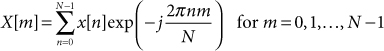
Because FT = N–1, the DFT from Eq. (MB 13.1) can be recast in terms of the sequence length N without any explicit appearance of the sampling interval T, or the frequency increment F:
MB 13.3

This formulation allows construction of generic DFT software routines that depend only upon the sequence length. In general, the frequency sequence, X[m], is complex-valued even in cases where the time sequence, x[n], is real-valued. However, when x[n] is an even-symmetric function in time, the corresponding DFT, X [m], is even-symmetric and real-valued. The roles of complex-valued time sequences are discussed in Note 60.
13.1. DFT Periodicity in the Frequency Domain
As discussed in Note 3, sampling in the time domain creates periodic spectral images in the frequency domain. How is this physical reality reflected in the mathematics of the DFT? In the equations that define the DFT, the frequency sequence, X[m], is defined only for 0 ≤ m < N. What happens if we try to generate X[m] for m ≥ N or for m < 0? Applying a few trigonometric identities and some algebraic manipulation to the DFT equations reveals that X[m + kN] = X[m] for k, an integer. In other words, if the index m is not constrained to the interval 0 ≤ m < N, the DFT produces a discrete frequency sequence that is periodic with a period of N samples, as illustrated in Figure 13.1. This periodicity is consistent with the physical results observed in real-world sampling experiments. The DFT in Eqs. (MB 13.1) and (MB 13.3) could be restated as being valid for all integer values of m. However, all of the useful spectral information is contained in a single period—the choice of the particular period corresponding to 0 ≤ m < N is somewhat arbitrary.
Figure 13.1. Implicit periodicity in the DFT spectrum. Solid drop lines indicate the “main” spectrum for 0 ≤ m ≤ (N – 1). Dashed drop lines indicate periodic replications of the “main” spectrum.

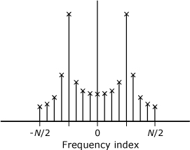
Despite an arbitrary choice of the period over which the DFT results are typically defined, periodicity in the results allows for some flexibility in how they are displayed. Consistent with the definitions (MB 13.1) and (MB 13.3), DFT results are often displayed for frequency indices from zero through N – 1. This format requires that the usual mathematical definitions of even and odd symmetry be recast to accommodate the fact that, in this format, the “negative” frequencies correspond to the indices, m, for (N/2) ≤ m < N. It is also fairly common to display results for frequency indices in the range ±N/2 using a “two-sided” format, as illustrated in Figure 13.2. This two-sided format is sometimes a more intuitive way to look at the frequency-domain symmetries. It should be noted that a two-sided plot involves N + 1 points because the point at m = N/2 is duplicated for m = –N/2.
Figure 13.2. Two-sided presentation of DFT spectrum
Math Box 13.2. Deriving the DFT from the DTFT
It is possible to create a DFT by applying the discrete-time Fourier transform (DTFT) to a finite-duration, discrete-time sequence, and evaluating the DTFT for only a finite set of specific discrete frequencies. The DTFT is defined in Note 12 as
MB 13.4
![]()
If we assume that x[n] is nonzero for only the N samples corresponding to n = 0, 1, . . ., N –1, then the summation limits in (MB 13.4) can be changed to yield
MB 13.5
![]()
However, X(ω) is still a function of continuous frequency, ω. If we attempt to define a DFT by evaluating Eq. (MB 13.5) at an arbitrary set of discrete frequencies, the result is generally not inverse-transformable back into the original sequence, x[n]. However, if we relax the constraints on x[n] somewhat, it becomes possible to obtain an invertible spectral representation that involves nonzero values at only N discrete frequencies. Specifically, we define xP[n] to be the periodic extension of x[n], such that the original N samples of x[n] comprise one period of the new periodic signal:
![]()
As discussed previously, sampling in the time domain leads to periodicity in the frequency domain, and periodicity in the time domain leads to sampling in the frequency domain. The DTFT of xP[n] is periodic, with a period equal to the original sampling frequency. Furthermore, due to the time-domain periodicity of xP[n], the DTFT is nonzero at only N discrete frequencies per period. Specifically, the discrete frequencies for the period occupying the interval 0 ≤ ω < T–1 is
![]()
Substituting ωm for ω in Eq. (MB 13.5) and converting to discrete sequence notation yields
which is the DFT defined by (MB 13.1).
13.2. Periodicity in the Time Domain
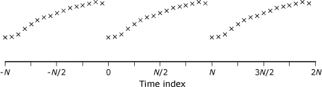
In the DSP literature, the DFT is described as operating on a time signal that is both discrete in time and also periodic, with a period of N samples. However, in the equations that define the DFT, values of the time sequence x[n] are needed only for values of n from 0 through N – 1; so why does it matter how x[n] behaves outside the interval 0 ≤ n < N? Furthermore, as given in Eq. (MB 13.2), the definition of the inverse DFT seems to imply that x[n] is defined only for values of n inside this interval. What does it really mean to say that the time signal that serves as input to the DFT is periodic?
The results produced by the DFT are as though the original N samples of x[n] have been duplicated along the time axis, as shown in Figure 13.3. In this periodic version of the signal, the sample at n = 0 is immediately preceded by a copy of the sample from n = N – 1, and the sample at n = N – 1 is immediately followed by a copy of the sample from n = 0. If there are discontinuities at these juxtaposed samples, the spectrum computed by the DFT may exhibit significant high-frequency content not present in the original signal. This spurious high-frequency content is sometimes called leakage. The usual technique for dealing with leakage is to multiply the time sequence by a window function that tapers the input sequence to values of zero or near zero at each end. This windowing technique effectively removes the discontinuities that cause leakage. Techniques for analyzing leakage are presented in Note 14, and leakage-reducing windows are discussed in Note 24.
Figure 13.3. Periodically extended presentation of DFT input record