
Note 24. Window Choices
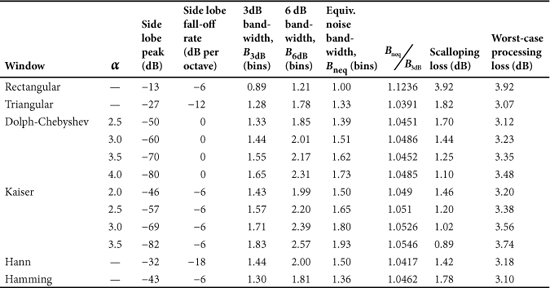
In this note, some of the more useful windows and some of the more commonly encountered windows are compared in terms of the characteristics discussed in Note 23. The characteristics of all windows discussed in this note are listed together in Table 24.1 for easy reference.
Table 24.1. Window Characteristics
24.1. Rectangular Window
The rectangular window is somewhat different from all of the other window functions in that rather than being explicitly applied to a data sequence, it instead represents the situation when a long or infinite sequence is truncated to form a shorter-duration segment. Modeling the truncation process as a windowing operation does provide a convenient mechanism for analyzing DFT leakage, as demonstrated in Note 15. The rectangular window is included in this note because it serves as a baseline from which the improvements offered by other windows can be gauged.
Truncating a DFT input sequence to a length of N samples can be mathematically modeled as multiplying the sequence by a rectangular window sequence that has non-zero values only for sample indices 0 through N – 1:
24.1
![]()
For a normalized sampling interval of T = 1, the DTFT of the rectangular window defined by Eq. (24.1) is given by
24.2
![]()
The exponential factor in (24.2) has a magnitude of 1 for all values of f, and represents a simple linear phase shift. This phase shift is a consequence of defining the window over the interval 0 ≤ n < N. If the rectangular window is defined to be symmetric about the origin, then the DTFT of the window is
24.3
![]()
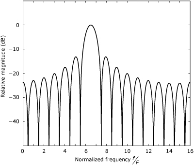
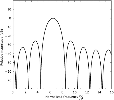
The DTFT magnitude response for a 16-point rectangular window is shown in Figure 24.1. The null-to-null width of the main lobe for the rectangular window is 2F, where F is the DFT bin spacing. The peaks of the first side lobes are about 13 dB below the peak of the main lobe. The ultimate side lobe attenuation is about 30 dB. As shown in Figure 24.1, the rectangular window’s response has nulls at all integer multiples of the frequency increment F = (NT)–1. This spacing of the nulls means that for a sinusoidal signal with a frequency of f = kF, the DFT has a non-zero response only in bins k and N – k. However, for a sinusoidal signal with a frequency that is not an integer multiple of F, the DFT exhibits some response in every bin. As shown in Figure 24.2, when the main lobe of the rectangular window’s response is centered on a frequency component that falls between two adjacent DFT bin frequencies, the main lobe straddles the two adjacent bins. When the signal is near the midpoint between two bins, the response in each of the two straddled bins is significant. However, as the signal is moved closer to one of the bins, the response in the other straddled bin becomes less significant.
Figure 24.1. DTFT magnitude response for a 16-point rectangular window
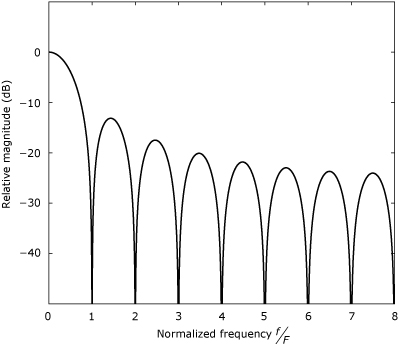
Figure 24.2. DTFT magnitude response for 16-point rectangular window, after shifting the center of the main lobe on a normalized frequency of 6.5
24.2. Triangular Window
The triangular window’s response has nulls at even-valued integer multiples of the DFT frequency increment. As shown in Figure 24.3, the side lobe peaks occur at frequencies very close to odd-valued integer multiples of the frequency increment. Furthermore, the null-to-null width of the main lobe in the response spans an interval of 4F. Therefore, when the triangular window’s response is centered on bin k, the responses at bins k – 1 and k + 1 are down only 7.8 dB from the peak. The responses at bins k ± 3 are down by about 26.7 dB from the peak at bin k. When the signal frequency is not an integer multiple of F, the main lobe straddles four consecutive DFT bins, as shown in Figure 24.4. The ultimate side lobe attenuation is about 48 dB.
Figure 24.3. DTFT magnitude response for a 16-point triangular window
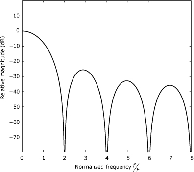
Figure 24.4. DTFT magnitude response for a 16-point triangular window after shifting to center the main lobe on a normalized frequency of 6.5
24.3. Dolph-Chebyshev Window
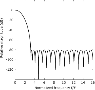
The Dolph-Chebyshev window has its origins in antenna design [2] and its response has the minimum main-lobe width for a given side lobe level. As depicted in Figure 24.5, all the side lobes peak at the same level. For a side lobe level of –20α, the window’s discrete-frequency response is given by
24.4
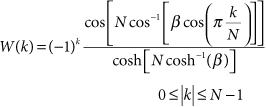
where
![]()
Figure 24.5. DTFT magnitude response for a 32-point Dolph-Chebyshev window
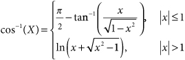
Often, β > 1 and, consequently, evaluation of Eq. (24.4) may entail computing the inverse cosine of values with magnitudes greater than unity. In such cases, the following formula can be used:
The time-domain window coefficients are obtained by taking the inverse DFT of Eq. (24.4).
24.4. Kaiser Window
The discrete-time Kaiser window is defined by
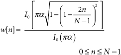
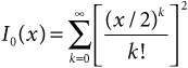
where I0 is the zero-order modified Bessel function of the first kind, given by
The Kaiser window is discussed further in Note 25, and its use in designing FIR filters is discussed in Note 36.
24.5. Hann Window
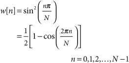
The discrete-time, odd-length Hann lag window is defined as

and the discrete-time (usually even-length) Hann data window is defined as
24.6. Hamming Window
The discrete-time, odd-length Hamming lag window is defined as
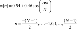
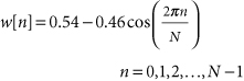
and the discrete-time (usually even-length) Hamming data window is defined as
References
1. f. j. harris, “On the use of Windows for Harmonic Analysis with the Discrete Fourier Transform,” Proc. IEEE, vol. 6, no. 1, pp. 51–83, January 1978.
2. C. L. Dolph, “A Current Distribution for Broadside Arrays Which Optimizes the Relationship Between Beam Width and Side-Lobe Level,” Proc. IRE, vol. 35, June 1946, pp. 335–348.