
Note 21. Using Window Functions: Some Fundamental Concepts
Within DSP, window usage can be divided into two broad categories: (1) windowing of signal segments to reduce leakage in the DFT, and (2) designing FIR filters that are based on using windows to reduce the Gibb’s phenomenon in finite approximations to ideal filters. Additional details concerning the use of windows for FIR filter design are discussed in Notes 23 and 24.
21.1. Elementary Windows
As discussed in Note 14, truncating a DFT input sequence to a length of N samples can be mathematically modeled as multiplying the sequence by a rectangular window sequence that has non-zero values only for sample indices 0 through N – 1
21.1
![]()
Rectangular windows are not particularly well suited for illustrating some of the time- and frequency-domain characteristics that make using windows so attractive. Therefore, we will begin by introducing a simple tapering window, called the triangular window, or sometimes, the Bartlett window.
Often, the mathematical descriptions of windows and their frequency responses are simplified if the window is defined centered around the zero index, as shown in Figure 21.1. A window in this position is sometimes called a lag window. It is natural to have an odd number of samples in a lag window so that one sample lies on the vertical axis and there are an equal number of samples to the left and to the right of the vertical axis. In this position, a triangular window can be defined as
21.2
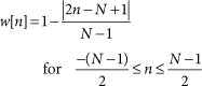
Figure 21.1. Triangular lag window with 33 points
As defined, this window has a value of zero at each end and a peak value of 1 in the center. It could be argued that this window really has a length of only N – 2 because of the two zero-valued endpoints. However, it is convenient for some analyses of window properties to include the zero-valued endpoints as part of the window. There are a number of different window families with similar concerns. Hann and Blackman windows are other commonly used windows that have zero-valued endpoints.
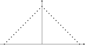
Different authors adopt different conventions with regard to how zero-valued endpoints are treated. For the case of triangular windows, MATLAB supports both approaches—the function triang(N) generates a triangular window having N nonzero values, and the function bartlett(N) generates a triangular window with zero-valued endpoints and N – 2 non-zero values. This support must be used with caution. For odd window lengths, as illustrated in Figure 21.2, for the case of N = 63, triang(N) produces a window that exactly equals the center N points of the window produced by bartlett(N+2). In other words, the result from triang(N) can be obtained just by removing the two zero-valued endpoints from the result produced by bartlett(N+2). In each case, the slope for the left side of the triangle is 1/32. However, this relationship between the results from triang(N) and bartlett(N+2) is not maintained for the case when N is even. As shown in Figure 21.3(a), in the window produced by bartlett(62), the peak of the triangle falls midway between sample indices 31 and 32. The left edge rises from a value of 0 at sample index 1, to a value of 1 at a point equivalent to sample index 31.5; thus the left-side slope is obtained as
![]()
Figure 21.2. Comparison of windows produced by MATLAB functions bartlett and triang for odd N
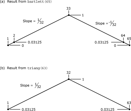
Figure 21.3. Comparison of windows produced by MATLAB functions bartlett and triang for even N
As shown in Figure 21.3(b), in the window produced by triang(60), the peak of the triangle falls midway between sample indices 30 and 31. Rather than having the first sample be equal to the first non-zero sample from bartlett(62) (which would locate the missing zero-valued samples at abscissae corresponding to sample indices 0 and 61), the implementers of MATLAB chose to construct the triangle in a way that places the zero values at abscissae corresponding to sample indices 0.5 and 60.5. This choice causes the left edge to rise from a value of 0 at a point equivalent to sample index 0.5, to a value of 1 at a point equivalent to sample index 30.5; thus the left-side slope is obtained as
![]()
21.2. Even-Length Windows for DFT Applications
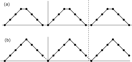
Even-length windows are most often used for reducing DFT leakage—the windows used in FIR filter design are usually odd in length. However, due to the implicit periodic extension inherent in the DFT, the correct way to generate the even-length windows used with even-length DFTs involves truncating the final point of an odd-length window. Figure 21.4(a) shows a symmetric 8-point triangular window and several of its images due to periodic extension. Figure 21.4(b) shows an asymmetric 8-point window that began as a symmetric 9-point window before the final point was truncated. As shown in the figure, the first point in each window image also fills the place of the missing final point for the preceding image.
Figure 21.4. Two different configurations for an even-length window: (a) naive approach, and (b) approach that exploits the periodic extension implicit in the DFT
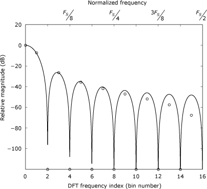
Looking at Figure 21.4, the difference between the two approaches might not seem important, but proper generation of the DFT window is crucial if the DFT results are to represent samples of the DTFT result. Figure 21.5 shows the positive-frequency DTFT spectrum for a 33-point triangular window with zero-valued endpoints (i.e., the results from bartlett(33) in MATLAB). Superimposed on the continuous trace of the DTFT spectrum are circles marking values from the DFT of the asymmetric 32-point window that results from truncating the final point of the original 33-point window. Figure 21.6 shows the DFT locations that result from the incorrect use of a 32-point symmetric window. The DFT locations are displaced from their correct locations, but they are close enough to explain why many practitioners are able to use even-length symmetric windows incorrectly and still obtain usable results.
Figure 21.5. Magnitude of DTFT for 33-point triangular window (solid trace) with magnitude of DFT for coresponding 32-point truncated windows (circles)
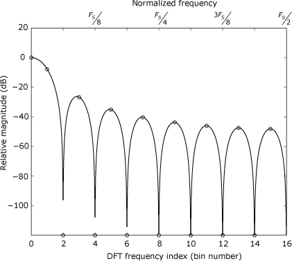
Figure 21.6. Magnitude of DTFT for 33-point triangular window (solid trace) with magnitude of DFT for symmetric 32-point window (circles)
21.3. Lobe Structure in the Frequency Response
There are four fundamental characteristics tied directly to the lobe structure of a window’s DTFT response.
- Width of the main lobe. The width can be specified as the null-to-null width or as the 3-dB or 6-dB bandwidth of the main lobe.
- Peak level of the first side lobe.
- Ultimate” attenuation of side lobes far removed from the main lobe. In the case of discrete-time windows, the ultimate attenuation is the attenuation at the side lobe peak closest to ω = π.
- Spacing of the nulls in the DTFT response.