Note 41. Chebyshev Filters
Chebyshev filters comprise one of the analog filter families that are commonly used as prototypes for IIR digital filters designed using either the impulse invariance method (Note 50) or the bilinear transformation (Note 51).
Alowpass Chebyshev filter is obtained as an equiripple approximation to the response of an ideal lowpass filter. This approximation yields a filter having a squared magnitude response given by
![]()
where
![]() 2 = 10r/20 –1
2 = 10r/20 –1
r = passband ripple
Tn(ω) = Chebyshev polynomial of order n
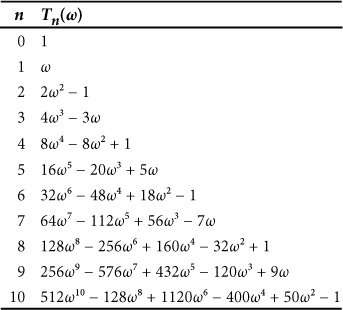
The first eleven Chebyshev polynomials are listed in Table 41.1. The table can be extended using the recurrence relation:
Tn+1(ω) = 2ωTn(w)–Tn–1(ω)
Table 41.1. Chebyshev Polynomials
Math Box 41.1. Chebyshev Transfer Function
The transfer function for an nth order Chebyshev LPF normalized for a ripple bandwidth equal to 1 is given by
MB 41.1
![]()
where
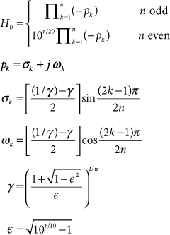
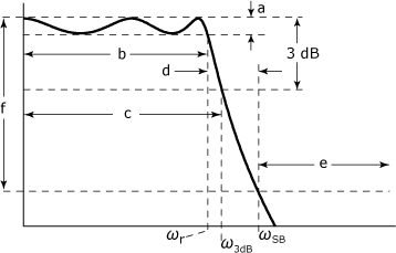
Figure 41.1 shows the important features in the magnitude response for a Chebyshev lowpass filter. The response is most often presented in a form where the response is normalized to have a ripple bandwidth, ωr, equal to 1, because this form involves simpler calculations. However, comparison with other filter families is often easier when the magnitude response is normalized to have the 3-dB frequency ω3dB equal to 1. Design Procedure 41.1 can be used to renormalize a filter design from ωr = 1 to ω3dB = 1. The transfer function for an nth order Chebyshev LPF normalized for ωr = 1 is given in Math Box 41.1.
Figure 41.1. Magnitude response of a fifth-order Chebyshev filter. Features are: (a) ripple limits, (b) ripple bandwidth, (c) 3-dB bandwidth, (d) transition band, (e) stopband, and (f) stopband attenuation.
Design Procedure 41.1. Renormalizing Chebyshev LPF Transfer Functions
Assuming that values of ε, H0, and the pole values pk have been obtained for a Chebyshev filter having a ripple bandwidth normalized to 1, this filter can be renormalized for a 3-dB bandwidth equal to 1 by performing the following steps.
- Compute A using
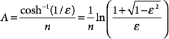
- Using the values of A obtained in step 1, compute R as
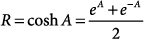
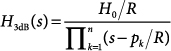
- Use R to compute H3dB(s) as
There are several different equations that can be used to estimate the minimum number of poles that are required for a Chebyshev lowpass filter to achieve a desired set of specifications. Two of the most commonly cited equations are from Rabiner and Gold [1]:
41.1
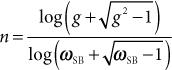

and from Van Valkenberg [2]:
41.2
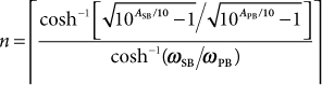
These two equations provide similar, but not identical, results. It’s worth noting that the MATLAB help file for the function cheb1ord() cites Rabiner and Gold, but Eq. (41.2) is used for the actual implementation contained in cheb1ord.m.
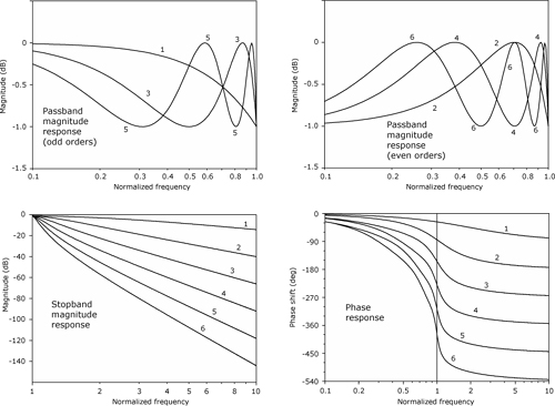
Figure 41.2 shows the magnitude and phase responses for lowpass Chebyshev filters of orders 1 through 6.
Figure 41.2. Frequency response plots for lowpass Chebyshev filters of orders 1 through 6
Design Procedure 41.2. Designing a Chebyshev Prototype
- Based on the requirements of the intended application, determine desired values for the following critical performance parameters to be exhibited by the final IIR design:
 = passband edge frequency based on ripple bandwidth
 = stopband edge frequency
ASB = minimum stopband attenuation
ε = passband ripple parameter
- Determine the prewarped frequencies, ω3dB and ωSB, corresponding to the desired final frequencies,
 and
and  . If the prototype is being designed for use in the bilinear transformation, the prewarped frequencies are given by
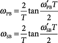
where T is the sampling interval for the IIR filter. If the prototype is being designed for use with the impulse invariance technique, there is no prewarping, so

- Determine the minimum filter order using either Eq. (41.1) or Eq. (41.2).
- Insert the value for ε from step 1, and the value for n from step 3 into Eq. (MB 41.1) to obtain the desired transfer function.
References
1. L. R. Rabiner and B. Gold, Theory and Applications of Digital Signal Processing, Prentice Hall, 1975.
2. M. E. Van Valkenberg, Analog Filter Design, Oxford University Press, 1982.
3. A. Antoniou, Digital Filters: Analysis and Design, McGraw-Hill, 1979.