Note 18. FFT: Decimation-in-Frequency Algorithms

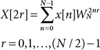
Decimation-in-time FFTs are based on repeatedly splitting the DFT summation into two summations—one for the decimated time sequence from which even-indexed samples have been removed and one for the decimated time sequence from which odd-indexed samples have been removed. As the name implies, decimation-in-frequency FFTs split the DFT summation in a way that produces decimated frequency sequences. The DFT summation can be specialized for computing only the even-indexed frequency samples:

18.1

After some algebraic manipulations, Eq. (18.1) can be put in the form

18.2

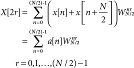
where a[n] is the sequence formed by adding together corresponding samples from the first and second halves of the original time sequence:

Thus, the even samples of the frequency sequence can be generated by performing an (N/2)-point DFT on combinations of samples from the original time sequence.

The DFT summation can also be specialized for computing only the odd-indexed frequency samples:

18.3

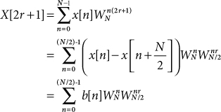
where b[n] is the sequence formed by subtracting samples in the second half of the original time sequence from the corresponding samples in the first half of the original time sequence:

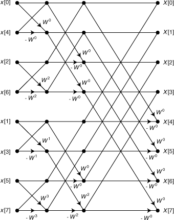
Thus, the odd samples of the frequency sequence can be generated by performing an (N/2)-point DFT on weighted combinations of samples from the original time sequence. The SFG corresponding to Eqs. (18.2) and (18.3) for the specific case of N = 8 is shown in Figure 18.1. If N = 2^L, the summations at each stage can be split. The SFG for N = 8 and L = 3 is shown in Figure 18.2. The input values appear in natural order from x[0] through x[7]. The output values appear in the bit-reversed order X[0], X[4], X[2], X[6], X[1], X[5], X[3], X[7]. It is possible to rearrange the nodes in Figure 18.2 without disturbing the connections between the nodes to obtain the SFG shown in Figure 18.3, where the inputs are in bit-reversed order and the outputs are in natural order.

Figure 18.1. Signal flow graph depicting operations defined by Eqs. (18.2) and (18.3)

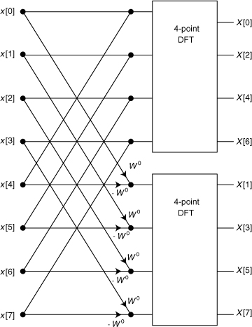
Figure 18.2. Signal flow graph for 8-point decimation-in-frequency FFT with naturally ordered inputs and permuted outputs

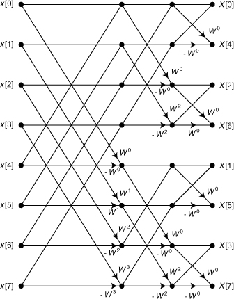
Figure 18.3. Signal flow graph for 8-point decimation-in-frequency FFT with permuted inputs and naturally ordered outputs