Note 68. Autoregressive Signal Models
Many real-world signals can be modeled as autoregressive (AR) processes. The properties of AR processes have led to the development of numerous techniques for analyzing and characterizing of such signals. This note serves as an introduction to these techniques, which are explored in subsequent notes.
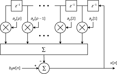
An autoregressive process of order p (often denoted as an “AR(p) process”) can be generated using a p-stage all-pole filter driven by a white noise source, as shown in Figure 68.1. The configuration shown in the figure implements the difference equation (68.1) given in Math Box 68.1, and is sometimes referred to as an autoregressive signal model.
Figure 68.1. All-pole filter configured for generating an AR(p) process
The AR model can be used in either a synthesis role or an analysis role. In the synthesis role, the model order p, the coefficients, b0 and ap[k], and the white noise variance, ![]() , are all assumed to be known, and the filter is used to generate the signal sequence, x[n], recursively. An example of the synthesis role is the implementation of a signal generator that produces a signal with particular statistical characteristics that might be needed for testing or simulation purposes.
, are all assumed to be known, and the filter is used to generate the signal sequence, x[n], recursively. An example of the synthesis role is the implementation of a signal generator that produces a signal with particular statistical characteristics that might be needed for testing or simulation purposes.
In the analysis role, a signal, x[n], is known for some values of n, and is assumed to be an auto regressive signal. The problem is to find values for ap[k] and ![]() that yield the estimated signal
that yield the estimated signal
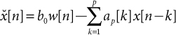
that is in some sense the “best” estimate for x[n]. In most cases where an AR signal model is used in an analysis role, the model’s filter coefficients are themselves the true goal of the effort, and the filter itself is never actually implemented. For example, Eq. (MB 68.3), given in Math Box 68.1, uses the filter coefficients to estimate the power spectral density of an autoregressive signal.
Math Box 68.1. Equations for Characterizing Autoregressive Processes
Difference Equation
MB 68.1
![]()
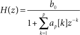
System Function
MB 68.2
Power Spectral Density
MB 68.3

References
1. M. H. Hayes, Statistical Digital Signal Processing and Modeling, Wiley, 1996.
2. N. Levinson, “The Wiener RMS (Root Mean Square) Error Criterion in Filter Design and Prediction,” J. Math Phys., vol. 25, 1947, pp. 261–278.
3. J. Durbin, “The Fitting of Time Series Models,” Rev. Inst. Int. Statist., vol. 28, 1960, pp. 233–243.