Note 59. Bandpass Sampling: Wedge Diagrams

From Note 58, we know that in bandpass sampling, the sampling rate, f_s, must satisfy

59.1

where m is an integer that satisfies

59.2

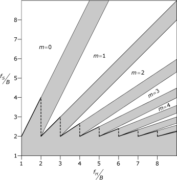
Many of the older discussions of bandpass sampling (such as [1]) include a diagram similar to Figure 59.1, which depicts only the lower bound imposed by Eq. (59.1). This diagram can be misleading to practitioners whose experience is limited to baseband sampling, where oversampling is often viewed as a good thing. It would be easy to select a sampling rate that satisfies the lower bound depicted in Figure 59.1, but that violates the upper bound imposed by Eq. (59.1). Vaughan, Scott, and White [2] appear to be the first authors to include a diagram similar to Figure 59.2, which depicts both the lower and upper bounds on the sampling rate given by Eq. (59.1).

Figure 59.1. Minimum normalized sampling rate for bandpass signals versus normalized band position

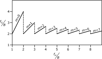
Figure 59.2. Plot of normalized sampling rate for bandpass signals versus normalized band position. The white areas indicate allowable combinations of sampling rate and band position. The shaded areas indicate combinations that exhibit aliasing.

In theory, we are free to choose any sampling rate that meets the constraints imposed by Eqs. (59.1) and (59.2). The largest choice of m allowed by Eq. (59.2) leads to the lowest sampling rates from Eq. (59.1), but choosing the largest m often can lead to a fragile sampling design. Section 59.2 explores how the choice of m can be best exploited for sampling designs that remain robust despite sample-clock inaccuracies and low-performance anti-aliasing filters often encountered in cost-conscious hardware designs.

59.1. Interpreting the Wedge Diagram

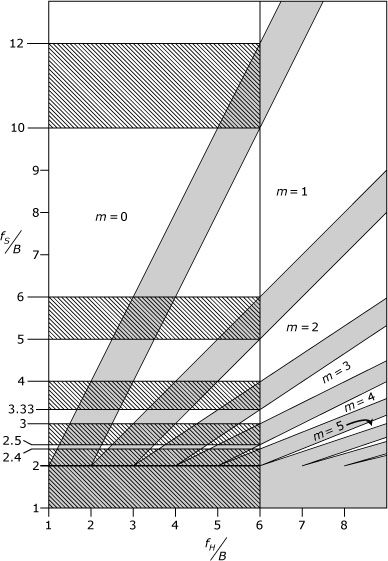
Figure 59.3 is a vertically extended copy of the wedge diagram from Figure 59.2 that has been annotated to illustrate the points raised in the following discussion regarding interpretation of the wedge diagram.

• Determine the band location, f_H, and bandwidth, B, for the signal that is to be sampled, and then draw a vertical line at the value corresponding to the ratio f_H/B. The portions of this line that pass through the various wedges define the range of sampling rates that can be used for sampling the signal. For example, if we draw a vertical line at f_H/B = 6, as shown in Figure 59.3, the line passes through the tip of the wedge for m = 5, and the corresponding ordinate is f_s = 2B. The line also passes through the interior of the wedges corresponding to all values of m < 5.

• Draw horizontal lines from the points where the vertical line intersects with the sloped lines that form the wedge boundaries. These horizontal lines intersect with the vertical axis at the values of f_s/B that bound each interval of legal sampling rates.

• As shown in the figure, a signal with f_H/B = 6 can be sampled at normalized rates, f_s/B, that fall within any of the intervals (2.4, 2.5), (3, 3.33), (4, 5), or (6, 10). The case for m = 0 corresponds to the baseband sample rate of f_S = 2f_H, or f_S/B = 12.

• If the actual value for the ratio f_H/B differs from the nominal value of 6, the resulting impact on the sampled signal would be as though the vertical line were shifted either left (if actual ratio is lower than 6) or right (if the actual ratio is higher than 6). This shifting might cause our selected operating point to move into the shaded area where aliasing occurs. The effects of errors in f_H/B are quantified in Section 59.2.

• Similarly, if the actual value for the normalized sampling rate, f_s/B, differs from the value corresponding to our selected operating point, the actual operating point can move up or down along the vertical line and possibly move into a shaded area where aliasing occurs.

Figure 59.3. Plot of normalized sampling rate for bandpass signals versus normalized band position. The white areas indicate allowable combinations of sampling rate and band position. The shaded areas indicate combinations that exhibit aliasing. The vertical line at f_H/B = 6 passes through white areas for f_s/B in the intervals (2.4, 2.5), (3, 3.33), (4, 5), and (6, 10).

59.2. Sensitivity to Timing Errors

The top of Figure 59.4 shows an enlarged portion of a single wedge taken from a diagram like the one shown in Figure 59.2. As discussed in the previous section, for given values of f_H and B, the operating point is placed inside one of the unshaded wedges somewhere on the vertical line that passes through the appropriate value of f_H/B.

Figure 59.4. Frequency relationships between the passbands of an original bandpass signal (shaded) and the images (unshaded) created by uniform bandpass sampling

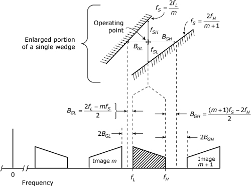
As shown in Figure 59.4, the operating point’s location within the wedge defines four quantities: f_SL, f_SH, B_GL, and B_GH. The operating point corresponds to some nominal sampling rate, f_s. The value of f_SL indicates how much the sample clock can fall below this nominal rate before the operating point moves into the lower shaded region and aliasing occurs. Similarly, the value of f_SH indicates how much the sample clock can increase above the nominal rate before the operating point moves into the upper shaded region and aliasing occurs.

The bottom of Figure 59.4 shows the positive-frequency portion of the spectrum from Figure 58.2 in Note 58. The spacing between the various images in this spectrum is related to the quantities, B_GL and B_GH, that are defined by the operating point’s horizontal distance from the wedge boundaries. The shaded band at the bottom of Figure 59.4 is the original signal’s positive-frequency band. The gap between this band and the mth image of the original negative-frequency band is 2B_GL, where B_GL is the horizontal distance from the operating point to the upper-left boundary of the wedge.

59.3

The gap between the shaded band and the (m + 1)-th image of the original negative-frequency band is 2B_GH, where B_GH is the horizontal distance from the operating point to the lower-right boundary of the wedge.

59.4

The empty intervals of length B_GL and B_GH surrounding each image band are sometimes referred to as guard bands.

References

1. R. S. Simpson and R. C. Houts, Fundamentals of Analog and Digital Communication Systems, Allyn and Bacon, 1971.

2. R. G. Vaughan, N. L. Scott, and D. L. White, “The Theory of Bandpass Sampling,” IEEE Trans. Signal Processing, vol. 39, no. 9, September 1991, pp. 1973–1984.