Note 38. Laplace Transform

The Laplace transform is a mathematical tool that is used primarily for analyzing linear analog systems such as filters. This transform is of interest in digital signal processing because analog filters having transfer functions defined in terms of Laplace transforms are often used as the starting point in the design of digital IIR filters. The characterization of analog filters is discussed in Note 39, and commonly used analog filter families are discussed in Notes 40 through 43.

The Laplace transform for a continuous-time function, x(t), is usually denoted as X(s) or L[x(t)], and is defined by Eq. (MB 38.1). The complex variable, s, is usually referred to as complex frequency, and can be put into the form σ + jω, where σ and ω are real variables, sometimes referred to as neper frequency and radian frequency, respectively.

Early interest in the Laplace transform was driven by the fact that if we take the Laplace transform of both sides of a differential equation in continuous time, t, we obtain an algebraic equation in complex frequency, s, that can be more easily solved for the desired quantity. The behavior of a linear analog filter is described by a differential equation in t, and consequently, the Laplace transform plays a big role in the analysis and characterization of analog filters.

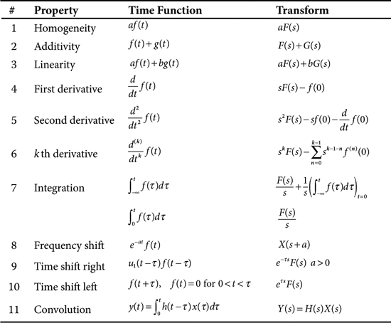
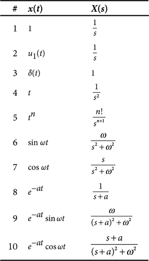
The inverse Laplace transform is defined by Eq. (MB 38.2). Evaluating the integrals in Eq. (MB 38.1) and, especially, Eq. (MB 38.2) can be a major chore. However, in practice, direct evaluation of these integrals usually can be avoided by using some well-known transform pairs selected from Table 38.1, along with a number of transform properties selected from Table 38.2.

Table 38.1. Laplace Transform Pairs

Table 38.2. Laplace Transform Properties