Note 70. Fitting All-Pole Models to Deterministic Signals: Autocorrelation Method

This note describes the autocorrelation method for finding the parameters needed to fit an all-pole model to a finite sequence of samples obtained from a deterministic signal. Although the genesis of each method is different, the autocorrelation method is compuatationally identical to the Yule-Walker method described in Note 69.

The autocorrelation method is a technique for fitting an all-pole model to a deterministic signal that is assumed to be autoregressive, but where knowledge about the signal is limited to a sequence of N samples, x[0] through x[N –1]. This technique is based on normal equations that result from perfroming an error minimization over the semi-infinite interval, 0 ≤ n, while assuming that the data sequence equals zero for n < 0 and for n ≥ N. Recipe 70.1 implements the autocorrelation method by using the Levinson-Durbin recursion to solve the normal equations that result from this particular error-minimization strategy.

70.1. Background

The all-pole model has the form

70.1

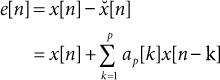
where the coefficients, a_p[k], are selected to minimize the error

70.2

with

70.3

Evaluation of Eq. (70.2) calls for some values of x[n] that fall outside of the known sequence, x[0] through x[N –1]. In the autocorrelation method, this difficulty is addressed by assuming that x[n] equals zero for n < 0 and for n ≥ N. Under this assumption, the normal equations become

70.4

where

70.5

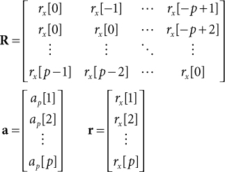
In matrix form, the normal equations are

70.6

where

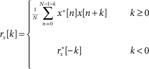
70.2. About Recipe 70.1

Equation (70.7) is the biased estimate of the ACS for finite N. The unbiased estimate is the same, except for a normalizing factor of 1/(N – k) that replaces the factor of 1/N. Normally, it is preferable to use unbiased rather than biased estimators, but for values of k that approach the value of N, the unbiased ACS estimator can produce results where the autocorelation estimate at lag zero is smaller than the estimate at one or more non-zero lags. This result can sometimes lead to matrix equations that cannot be solved [4]. Therefore, the biased ACS estimate is almost always the one used in the autocorrelation method.

Along the way to producing the coefficients, a_p[i], for an AR(p) model, the Levinson recursion generates coefficients for all of the lesser-order models, AR(1) through AR(p –1).

References

1. M. H. Hayes, Statistical Digital Signal Processing and Modeling, Wiley, 1966.

2. N. Levinson, “The Wiener RMS (Root Mean Square) Error Criterion in Filter Design and Prediction,” J. Math Phys., vol. 25, 1947, pp. 261–278.

3. J. Durbin, “The Fitting of Time Series Models,” Rev. Inst. Int. Statist., vol. 28, 1960, pp. 233–243.

4. S. L. Marple, Digital Spectral Analysis with Applications, Prentice Hall, 1987.