Note 60. Complex and Analytic Signals

An understanding of complex and analytic signals is an essential foundation for the development of many advanced signal processing techniques.

A real-valued signal always has a magnitude spectrum that is symmetric about f = 0, as depicted in Figure 60.1(a). Many different digital receiver architectures depend upon the abilities to (1) eliminate either all of the positive-frequency content or all of the negative-frequency content in such a signal’s spectrum, and then (2) shift the surviving spectral band so that it is concentrated around zero frequency, as shown in Figure 60.1(c). A continuous-time signal having a spectrum that is zero-valued for all negative frequencies, as in Figure 60.1(b), is called an analytic signal because it can be represented mathematically as an analytic function [1].

Figure 60.1. Spectra at different points in a digital receiver architecture: (a) spectrum for real-valued bandpass intermediate-frequency (IF) signal, (b) spectrum for the IF signal’s analytic associate, (c) spectrum for complex-valued baseband signal

This note first explores how the concepts of analytic signals can be extended to discrete-time signals and then it provides an overview of the various techniques for generating discrete-time analytic-like¹ signals. Each of these techniques is explored in depth in subsequent notes.

For any real-valued signal, x(t), the corresponding analytic signal, x_a(t), can be formed as

60.1

where H{·} denotes the Hilbert transform². Multiplication by j is equivalent to a phase shift of 90 degrees, so the net combined effect of jH{·} in Eq. (60.1) is to create a phase shift of zero for positive frequencies in the spectrum of x(t), and a phase shift of 180 degrees for negative frequencies in the spectrum of x(t). When jH{x(t)} is added to x(t), the negative-frequency components cancel and the positive-frequency components are doubled. If an analytic signal, x_a(t), is formed using Eq. (60.1), it is possible to recover the original signal, x(t), by simply taking the real part of x_a(t)

A real-valued signal exhibits conjugate symmetry in its Fourier spectrum. Therefore, any signal not exhibiting conjugate symmetry in its spectrum must be complex-valued in time. This means that analytic signals and conjugate-analytic signals are always complex-valued in time. However, there can be signals that are complex-valued in time but that are neither analytic nor conjugate-analytic. A handy example is the complex-valued baseband signal having the spectrum depicted in Figure 60.1(c). The spectrum is not zero for either positive or negative frequencies, so the signal is neither analytic nor conjugate-analytic. However, the magnitude spectrum is not symmetric about f = 0, so the signal is complex-valued.

60.1. Discrete-Time Analytic Signals

The concept of an analytic signal cannot be extended directly from the continuous-time domain to the discrete-time domain. The DTFT spectrum of a discrete-time signal is always periodic, so it is not possible for the spectrum to be non-zero for positive frequencies and zero for all negative frequencies simultaneously. For discrete-time signals, the concept of analyticity is based on a DTFT spectrum like the one shown in Figure 60.2, where the spectrum is non-zero in all odd-numbered positive Nyquist zones³ as well as in all even-numbered negative Nyquist zones. A discrete-time signal with such a spectrum is conventionally called an analytic signal, even though it cannot be represented as an analytic function. As noted previously, we follow Marple’s practice and distinguish the discrete-time case as being analytic-like. Furthermore, we use positive-like to indicate frequencies in odd-numbered positive Nyquist zones and in even-numbered negative Nyquist zones. Similarly, we use negative-like to indicate frequencies in odd-numbered negative Nyquist zones and in even-numbered positive Nyquist zones.

Figure 60.2. DTFT spectra for: (a) the original discrete-time, real-valued bandpass signal, and (b) the complex-valued analytic associate of the original signal

60.2. Generating Analytic Signals

There are a number of different techniques that can be used to generate an analytic signal. The following sections introduce five of the most useful approaches.

Spectrum Tailoring Approach

The spectrum tailoring approach can be used to generate the analytic-like associate by forcing the spectrum to zero for negative-like frequencies. Recipe 60.1 lists the strategy for spectrum tailoring. However, this is just a conceptual strategy; it should not be implemented directly. A practical algorithm is a bit more complicated.

Any frequency-domain operation that is performed on a signal’s DFT spectrum corresponds to some sort of time-domain filtering operation that could, in theory, be applied directly to the time-domain signal. In most cases, this filtering operation has a unit sample response that is longer than one sample in duration. Even in cases where the filter is defined directly in the frequency domain, and we do not know or need the corresponding unit sample response, we must make allowances for the length of this response by using the fast convolution technique described in Note 20. If we were to apply the three-step strategy listed above directly, the resulting analytic-like signal would, in most cases, exhibit time-domain aliasing.

Recipe 60.2 is the result of modifying Recipe 20.1 to implement spectrum tailoring. There are a few nuances in step 3 that might need further explanation. The point at m = N/2 sits on the transition from positive-like frequency to negative-like frequency and it is not immediately obvious why X_a[N/2] is not set to either 0 or 2X[N/2] rather than to X[N/2]. However, in [1], Marple shows that setting X_a[N/2] = X[N/2] is necessary to satisfy properties 1 and 2 from Math Box 60.1.

The MATLAB function hilbert uses an approach described in [3] that is equivalent to the approach detailed in Recipe 60.1, but that does not include the anti-aliasing measures embodied in Recipe 60.2. When using MATLAB, these measures must be implemented via vector manipulations external to the hilbert function. This function might have been more aptly named analytic, because y=hilbert(x) returns a complex vector that contains the analytic-like associate of x; the Hilbert transform of x must be obtained by taking the imaginary part of y.

Hilbert Transform Approach

It is possible to generate an analytic sequence using a “discretized” version of Eq. (60.1). For any real-valued signal sequence, x[n], the corresponding “analytic” sequence, x_a[n], can be formed as

60.2

where H[·] denotes the discrete Hilbert transform. An ideal discrete Hilbert transformer is a discrete-time filter having an impulse response, h[n], and transfer function, H(e^jω), given by

60.3

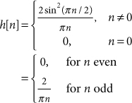
60.4

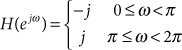
An ideal Hilbert transformer is not realizable, so practical implementations for generating analytic-like discrete-time signals must be built around approximations to the ideal Hilbert transformer. These approximations insert delay in Im{x_a[n]}, so Re{x_a[n]} must be delayed by a corresponding amount. Design of FIR Hilbert transformers is covered in Note 61.

Frequency-Shifted Lowpass Filters

A useful technique for designing FIR analytic signal generating filters is presented by Reilly et. al. in [4]. The basic idea is to design a “standard” lowpass filter having real-valued coefficients, and then phase-shifts the impulse response coefficients such that the filter’s passband is shifted to cover only positive frequencies and the stopband is shifted to cover only negative frequencies. This approach is explored further in Note 62.

Paired-Filter Approach

The key that makes Eq. (60.1) work is that x[n] and jH[x[n]] have spectra that are inphase for positive-like frequencies and 180 degrees out of phase for negative-like frequencies. A similar phasing relationship can be exploited to generate an analytic-like signal using an alternative approach that does not require a Hilbert transformer. Specifically, the analytic-like signal is formed as

60.5

where, ideally, P and Q are all-pass filters that are designed to have phase responses such that the phase of Q lags the phase of P by 90 degrees for all positive-like frequencies, and the phase of Q leads the phase of P by 90 degrees for all negative-like frequencies. Then when multiplication by j advances the phase of Q{x[n]} by 90 degrees, the phases of P{x[n]} and jQ{x[n]} are inphase for positive-like frequencies and 180 degrees out of phase for negative-like frequencies. Sometimes, the network comprising the two filters P and Q is referred to as an analytic-signal generating filter, or ASG filter. Design of IIR filter pairs for P and Q, as used in Eq. (60.4), is discussed and demonstrated in Note 63.

Complex Filter Approach

It is possible to design a single complex-valued filter that generates the analytic associate of the signal applied to the filter’s input. One way to design such a filter involves the complex extension of the Parks-McClellan algorithm. Design of complex-valued ASG filters using this extended algorithm is discussed in Note 64.

References

1. S. L. Marple, “Computing the Discrete-Time ‘Analytic’ Signal via FFT,” IEEE Trans. Signal Proc., vol. 47, no. 9, September 1999, pp. 2600–2603.

2. B. Boashash, Time Frequency Signal Analysis and Processing: A Comprehensive Reference, Elsevier, 2003.

3. hilbert help article from MATLAB help system.

4. A. Reilly, G. Frazer, and B. Boashash, “Analytic Signal Generation—Tips and Traps,” IEEE Trans. Signal Proc., vol. 42, no. 11, Nov. 1994, pp. 3241–3245.